Linear Diffusion Flows
This tours studies linear diffusion PDEs, a.k.a. the heat equation. A good reference for diffusion flows in image processing is [Weickert98].
Contents
Installing toolboxes and setting up the path.
You need to download the following files: signal toolbox and general toolbox.
You need to unzip these toolboxes in your working directory, so that you have toolbox_signal and toolbox_general in your directory.
For Scilab user: you must replace the Matlab comment '%' by its Scilab counterpart '//'.
Recommandation: You should create a text file named for instance numericaltour.sce (in Scilab) or numericaltour.m (in Matlab) to write all the Scilab/Matlab command you want to execute. Then, simply run exec('numericaltour.sce'); (in Scilab) or numericaltour; (in Matlab) to run the commands.
Execute this line only if you are using Matlab.
getd = @(p)path(p,path); % scilab users must *not* execute this
Then you can add the toolboxes to the path.
getd('toolbox_signal/');
getd('toolbox_general/');
Heat Diffusion
The heat equation reads \[ \forall t>0, \quad \pd{f_t}{t} = \nabla f_t \] for a function \(f_t : \RR^2 \rightarrow \RR\) and where \(f_0\) (the solution at initial time \(t=0\)) is given.
The Laplacian operator reads \[ \Delta f = \pdd{f}{x_1} + \pdd{f}{x_2}. \]
The flow is discretized in space by considering a discrete image of \(N = n \times n\) pixels.
n = 256;
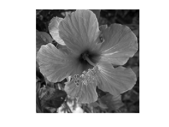
Load an image \(f_0 \in \RR^N\), that will be used to initialize the flow at time \(t=0\).
name = 'hibiscus';
f0 = load_image(name,n);
f0 = rescale( sum(f0,3) );
Display it.
clf;
imageplot(f0);
The flow is discretized in time using an explicit time-stepping \[ f^{(\ell+1)} = f^{(\ell)} + \tau \Delta f^{(\ell)}. \] We use finite difference Laplacian \[ (\Delta f)_i = \frac{1}{h^2}\pa{ f_{i_1+1,i_2}+f_{i_1-1,i_2}+f_{i_1,i_2+1}+f_{i_1,i_2-1}-4f_j }\] where we assume periodic boundary conditions, and where \(h = 1/N\) is the spacial step size.
h = 1/n;
delta = @(f)1/h^2 * div(grad(f));
The step size \(\tau\) should satisfy \[ \tau < \frac{h^2}{4} \] for the discretized flow to be stable.
The discrete solution \(f^{(\ell)}\) converges to the continuous solution \(f_t\) at time \(t = \tau \ell\) if both \(\tau \rightarrow 0\) and \(h \rightarrow 0\) under the condition \(\tau/h^2 < 1/4\).
Select a small enough step size.
tau = .5 * h^2/4;
Final time.
T = 1e-3;
Number of iterations.
niter = ceil(T/tau);
Initialize the diffusion at time \(t=0\).
f = f0;
One step of discrete diffusion.
f = f + tau * delta(f);
Exercice 1: (check the solution) Compute the solution to the heat equation.
exo1;

Explicit Solution using Convolution
The solution to the heat equation can be computed using a convolution \[ \forall t>0, \quad f_t = f_0 \star h_t \] where \(\star\) denotes the convolution of continuous functions \[ f \star h(x) = \int_{\RR^2} f(y) g(x-y) d y \] and \(h_t\) is a Gaussian kernel of width \(\sqrt{t}\) \[ h_t(x) = \frac{1}{4 \pi t} e^{ -\frac{\norm{x}^2}{4t} } \]
One can thus approximate the solution using a discrete convolution. Convolutions can be computed in \(O(N\log(N))\) operations using the FFT, since \[ g = f \star h \qarrq \forall \om, \quad \hat g(\om) = \hat f(\om) \hat h(\om). \]
cconv = @(f,h)real(ifft2(fft2(f).*fft2(h)));
Define a discrete Gaussian blurring kernel of width \(\sqrt{t}\).
t = [0:n/2 -n/2+1:-1];
[X2,X1] = meshgrid(t,t);
normalize = @(h)h/sum(h(:));
h = @(t)normalize( exp( -(X1.^2+X2.^2)/(4*t) ) );
Define blurring operator.
heat = @(f, t)cconv(f,h(t));
Example of blurring.
clf;
imageplot(heat(f0,2));

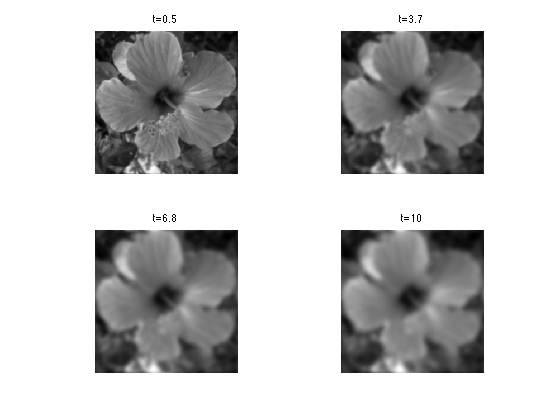
Exercice 2: (check the solution) Display the heat convolution for increasing values of \(t\).
exo2;
Bibliography
- [Weickert98] Joachim Weickert, Anisotropic Diffusion in Image Processing, ECMI Series, Teubner-Verlag, Stuttgart, Germany, 1998.