\[ \newcommand{\NN}{\mathbb{N}} \newcommand{\CC}{\mathbb{C}} \newcommand{\GG}{\mathbb{G}} \newcommand{\LL}{\mathbb{L}} \newcommand{\PP}{\mathbb{P}} \newcommand{\QQ}{\mathbb{Q}} \newcommand{\RR}{\mathbb{R}} \newcommand{\VV}{\mathbb{V}} \newcommand{\ZZ}{\mathbb{Z}} \newcommand{\FF}{\mathbb{F}} \newcommand{\KK}{\mathbb{K}} \newcommand{\UU}{\mathbb{U}} \newcommand{\EE}{\mathbb{E}} \newcommand{\Aa}{\mathcal{A}} \newcommand{\Bb}{\mathcal{B}} \newcommand{\Cc}{\mathcal{C}} \newcommand{\Dd}{\mathcal{D}} \newcommand{\Ee}{\mathcal{E}} \newcommand{\Ff}{\mathcal{F}} \newcommand{\Gg}{\mathcal{G}} \newcommand{\Hh}{\mathcal{H}} \newcommand{\Ii}{\mathcal{I}} \newcommand{\Jj}{\mathcal{J}} \newcommand{\Kk}{\mathcal{K}} \newcommand{\Ll}{\mathcal{L}} \newcommand{\Mm}{\mathcal{M}} \newcommand{\Nn}{\mathcal{N}} \newcommand{\Oo}{\mathcal{O}} \newcommand{\Pp}{\mathcal{P}} \newcommand{\Qq}{\mathcal{Q}} \newcommand{\Rr}{\mathcal{R}} \newcommand{\Ss}{\mathcal{S}} \newcommand{\Tt}{\mathcal{T}} \newcommand{\Uu}{\mathcal{U}} \newcommand{\Vv}{\mathcal{V}} \newcommand{\Ww}{\mathcal{W}} \newcommand{\Xx}{\mathcal{X}} \newcommand{\Yy}{\mathcal{Y}} \newcommand{\Zz}{\mathcal{Z}} \newcommand{\al}{\alpha} \newcommand{\la}{\lambda} \newcommand{\ga}{\gamma} \newcommand{\Ga}{\Gamma} \newcommand{\La}{\Lambda} \newcommand{\Si}{\Sigma} \newcommand{\si}{\sigma} \newcommand{\be}{\beta} \newcommand{\de}{\delta} \newcommand{\De}{\Delta} \renewcommand{\phi}{\varphi} \renewcommand{\th}{\theta} \newcommand{\om}{\omega} \newcommand{\Om}{\Omega} \renewcommand{\epsilon}{\varepsilon} \newcommand{\Calpha}{\mathrm{C}^\al} \newcommand{\Cbeta}{\mathrm{C}^\be} \newcommand{\Cal}{\text{C}^\al} \newcommand{\Cdeux}{\text{C}^{2}} \newcommand{\Cun}{\text{C}^{1}} \newcommand{\Calt}[1]{\text{C}^{#1}} \newcommand{\lun}{\ell^1} \newcommand{\ldeux}{\ell^2} \newcommand{\linf}{\ell^\infty} \newcommand{\ldeuxj}{{\ldeux_j}} \newcommand{\Lun}{\text{\upshape L}^1} \newcommand{\Ldeux}{\text{\upshape L}^2} \newcommand{\Lp}{\text{\upshape L}^p} \newcommand{\Lq}{\text{\upshape L}^q} \newcommand{\Linf}{\text{\upshape L}^\infty} \newcommand{\lzero}{\ell^0} \newcommand{\lp}{\ell^p} \renewcommand{\d}{\ins{d}} \newcommand{\Grad}{\text{Grad}} \newcommand{\grad}{\text{grad}} \renewcommand{\div}{\text{div}} \newcommand{\diag}{\text{diag}} \newcommand{\pd}[2]{ \frac{ \partial #1}{\partial #2} } \newcommand{\pdd}[2]{ \frac{ \partial^2 #1}{\partial #2^2} } \newcommand{\dotp}[2]{\langle #1,\,#2\rangle} \newcommand{\norm}[1]{|\!| #1 |\!|} \newcommand{\normi}[1]{\norm{#1}_{\infty}} \newcommand{\normu}[1]{\norm{#1}_{1}} \newcommand{\normz}[1]{\norm{#1}_{0}} \newcommand{\abs}[1]{\vert #1 \vert} \newcommand{\argmin}{\text{argmin}} \newcommand{\argmax}{\text{argmax}} \newcommand{\uargmin}[1]{\underset{#1}{\argmin}\;} \newcommand{\uargmax}[1]{\underset{#1}{\argmax}\;} \newcommand{\umin}[1]{\underset{#1}{\min}\;} \newcommand{\umax}[1]{\underset{#1}{\max}\;} \newcommand{\pa}[1]{\left( #1 \right)} \newcommand{\choice}[1]{ \left\{ \begin{array}{l} #1 \end{array} \right. } \newcommand{\enscond}[2]{ \left\{ #1 \;:\; #2 \right\} } \newcommand{\qandq}{ \quad \text{and} \quad } \newcommand{\qqandqq}{ \qquad \text{and} \qquad } \newcommand{\qifq}{ \quad \text{if} \quad } \newcommand{\qqifqq}{ \qquad \text{if} \qquad } \newcommand{\qwhereq}{ \quad \text{where} \quad } \newcommand{\qqwhereqq}{ \qquad \text{where} \qquad } \newcommand{\qwithq}{ \quad \text{with} \quad } \newcommand{\qqwithqq}{ \qquad \text{with} \qquad } \newcommand{\qforq}{ \quad \text{for} \quad } \newcommand{\qqforqq}{ \qquad \text{for} \qquad } \newcommand{\qqsinceqq}{ \qquad \text{since} \qquad } \newcommand{\qsinceq}{ \quad \text{since} \quad } \newcommand{\qarrq}{\quad\Longrightarrow\quad} \newcommand{\qqarrqq}{\quad\Longrightarrow\quad} \newcommand{\qiffq}{\quad\Longleftrightarrow\quad} \newcommand{\qqiffqq}{\qquad\Longleftrightarrow\qquad} \newcommand{\qsubjq}{ \quad \text{subject to} \quad } \newcommand{\qqsubjqq}{ \qquad \text{subject to} \qquad } \]

Fenchel-Rockafellar Duality

This numerical tour is an introduction to convex duality with an application to total variation denoising.

Convex Duality
FB on the Fenchel-Rockafellar Dual Problem
Total Variation
Total Variation Regularization
Chambolle Dual Algorithm

Convex Duality

Given some convex, proper, and lower semi-continuous function \(f(x)\) defined for \(x \in \RR^N\), its Legendre-Fenchel dual function is defined as \[ \forall u \in \RR^N, \quad f^*(u) = \umax{x \in \RR^N} \dotp{x}{u} - f(x). \]

One can show that \(f^*\) is a convex function, and that it satisfies \((f^*)^* = f\).

One can show if \(f(x) = \frac{1}{2} \norm{A x - b}^2\) where \(A \in \RR^{N \times N}\) is an invertible matrix, then \[f^*(u) = \frac{1}{2} \norm{\tilde A u + b}^2 \qwhereq \tilde A = (A^*)^{-1}. \]

One can show that in the case of \(\ell^p\) norms \[ f(x) = \norm{x}_p = \pa{ \sum_{i=1}^N \abs{x_i}^p }^{1/p} \] with the usual extension to \(p=+\infty\) \[ \norm{x}_\infty = \umax{1 \leq i \leq N} \abs{x_i}\] then one has \[ f^*(u) = \iota_{\norm{\cdot}_q \leq 1} \qwhereq \frac{1}{p}+\frac{1}{q}=1, \] where \(\iota_{\Cc}\) is the indicator function of the convex set \(\Cc\).

FB on the Fenchel-Rockafellar Dual Problem

We are concerned with the minimization of composite problems of the form \[ \umin{x \in \RR^N} f(x) + g(A(x)) \] where \( A \in \in \RR^{P \times N} \) is a linear map (a matrix), \(f : \RR^N \rightarrow \RR \) and \(g : \RR^P \rightarrow \RR \) are convex functional.

We now assume that \(f\) is a \(L\)-strongly convex function. In this case, one can show that \(f^*\) is a \(C^1\) smooth function, and that its gradient is \(L\)-Lipschitz.

In this case, the Fenchel-Rockafellar theorem shows that one can solve the following dual problem \[ \umin{x \in \RR^N} f(x) + g(A(x)) = - \umin{u \in \RR^P} f^*( -A^* u ) + g^*(u) \] and recover the unique solution \(x^\star\) of the primal problem from a (non-necessarily unique) solution \(u^\star\) to the dual problem as \[ x^\star = \nabla f^*( -A^* u^\star ). \]

Denoting \(F(u) = f^*( -A^* u )\) and \(G(u) = g^*(u)\), one thus needs to solve the problem \[ \umin{u \in \RR^P} F(u) + G(u). \]

We assume that the function \(g\) is simple, in the sense that one can compute in closed form the so-called proximal mapping, which is defined as \[ \text{prox}_{\ga g}(x) = \uargmin{z \in \RR^N} \frac{1}{2}\norm{x-z}^2 + \ga g(z). \] for any \(\ga > 0\).

Note that \(g\) being simple is equivalent to \(g^*\) also being simple because of Moreau's identity: \[ x = \text{prox}_{\tau g^*}(x) + \tau \text{prox}_{g/\tau}(x/\tau). \]

Since \(F\) is smooth and \(G\) is simple, one can apply the Foward-Backward algorithm, which reads, after initilizing \(u^{(0)} \in \RR^P\), \[ u^{(\ell+1)} = \text{prox}_{\ga G}\pa{ u^{(\ell)} - \ga \nabla F( u^{(\ell)} ) }. \] with \(\ga < 2/L\).

The primal iterates are defined as \[ x^{(\ell)} = \nabla F( -A^* u^{(\ell)} ). \]

Total Variation

The total variation of a smooth function \( \phi : \RR^2 \rightarrow \RR \) is defined as \[ J(\phi) = \int \norm{\nabla \phi(s)} d s\] The total variation of an image is also equal to the total length of its level sets. \[ J(\phi) = \int_{-\infty}^{+\infty} L( S_t(\phi) ) dt. \] Where \(S_t(\phi)\) is the level set at \(t\) of the function \(\phi\) \[S_t(\phi)= \enscond{ s }{ \phi(s)=t } . \] This shows that the total variation can be extended to functions having step discontinuities.

We consider images \(x = (x_{i,j})_{i,j} \in \RR^N\) of \(N=n\times n\) pixels.

We consider here a discretized gradient operator \( A : \RR^N \rightarrow \RR^P \) where \(P=2N\) defined as \[ A x = u = (u^1,u^2) \qwhereq u^1 = ( x_{i+1,j}-x_{i,j} )_{ i,j } \in \RR^N \qandq u^2 = ( x_{i,j+1}-x_{i,j} )_{ i,j } \in \RR^N. \] where we assume periodic boundary conditions for simplicity.

A = @(x)grad(x);

The adjoint \(A^*\) of the discrete gradient is minus the discrete divergence.

As = @(u)-div(u);

In the following, while images \(x \in \RR^{N}\) are stored as arrays of size (n,n), gradient vector fields \(u \in \RR^P\) are stored as arrays size (n,n,2).

The discrete total variation is defined as the \(\ell^1-\ell^2\) norm of the discretized gradient \[ J(x) = \norm{A x}_{1,2} \qwhereq \norm{u}_{1,2} = \sum_{i,j} \norm{u_{i,j}} \] where \(u = (u_{i,j} \in \RR^2)_{i,j}\) is a vector field.

norm12 = @(u)sum(sum( sqrt(sum( u.^2,3 )) ));
J = @(x)norm12(A(x));

Total Variation Regularization

We consider here denoising using total variation regularization. This was first introduced in:

L.I. Rudin, S. Osher, E. Fatemi, Nonlinear total variation based noise removal algorithms, Physica D, vol. 60, pp. 259-268, 1992.

Given a noisy image \(y \in \RR^N\), it computes \[ x^\star = \uargmin{x \in \RR^N} \frac{1}{2}\norm{x-y}^2 + \la J(x), \] where the regularization parameter \(\la \geq 0\) should be adapted to the noise level.

Number of pixels.

n = 256;

First we load an image \(x_0 \in \RR^N\) of \(N=n \times n\) pixels.

name = 'hibiscus';
x0 = load_image(name,n);
x0 = rescale( sum(x0,3) );

Display the original image \(x_0\).

clf;
imageplot(clamp(x0));

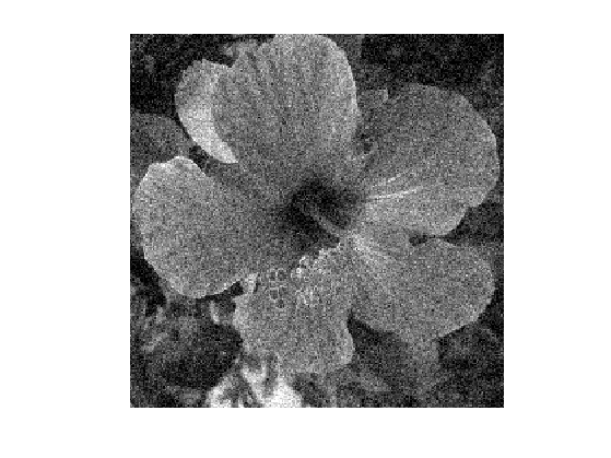
Add some noise to the original image, to obtain \(y=x0+w\).

sigma = .1;
y = x0 + randn(n,n)*sigma;

Display the noisy image \(y\).

clf;
imageplot(clamp(y));

Set the regularization parameter \(\la\).

lambda = .2;

Chambolle Dual Algorithm

We consider here the application of FB on the dual of the ROF problem, as initially proposed in:

Antonin Chambolle, An Algorithm for Total Variation Minimization and Applications, Journal of Mathematical Imaging and Vision, 20(1-2), 2004.

An earlier version of this algorithm was proposed in:

B. Mercier, Inequations Variationnelles de la Mecanique Publications Mathematiques d'Orsay, no. 80.01. Orsay, France, Universite de Paris-XI, 1980.

For a description of a more general framework, see:

P. L. Combettes, Dinh Dung, and B. C. Vu, Dualization of signal recovery problems, Set-Valued and Variational Analysis, vol. 18, pp. 373-404, December 2010

The primal problem corresponds to minimizing \(E(x) = f(x)+g(A(x))\) where \[ f(x) = \frac{1}{2}\norm{x-y}^2 \qandq g(u) = \la \norm{u}_{1,2}. \]

mynorm = @(x)norm(x(:));
f = @(x)1/2*mynorm(x-y)^2;
g = @(x)lambda*J(x);
E = @(x)f(x)+g(x);

The dual problem corresponds to minimzing \(F(u)+ G(u)\) where \[ F(u) = \frac{1}{2} \norm{y - A^* u}^2 - \frac{1}{2}\norm{y}^2 \qandq G(u) = \iota_{\Cc}(u) \qwhereq \Cc = \enscond{u}{\norm{u}_{\infty,2} \leq \la}. \] where \[ \norm{u}_{\infty,2} = \umax{i,j} \norm{u_{i,j}} \]

F = @(u)1/2*mynorm(y-As(u))^2 - 1/2*mynorm(y)^2;

One can thus solves the ROF problem by computing \[ x^\star = y - A^* u^\star \] where \[ u^\star \in \uargmin{ \norm{u}_{1,2} \leq \la } \norm{y - A^* u} \]

One can compute explicitely the gradient of \(F\): \[ \nabla F(u) = A (A^* u - y). \]

nablaF = @(u)A(As(u)-y);

The proximal operator of \( G \) is the orthogonal projection on \(\Cc\), which is obtained as \[ \text{prox}_{\ga G}(u)_{i,j} = \frac{u_{i,j}}{ \max(1,\norm{u_{i,j}}/\lambda) }. \] Note that it does not depends on \(\ga\).

d = @(u)repmat( sqrt(sum(u.^2,3)), [1 1 2] );
proxG = @(u,gamma)u ./ max( d(u)/lambda, 1 );

The gradient step size of the FB should satisfy \[ \ga < \frac{2}{\norm{A^* A}} = \frac{1}{4}. \]

gamma = 1/5;

Initialize the FB with \(u=0 \in \RR^P\).

u = zeros(n,n,2);

One step of FB.

u = proxG( u - gamma * nablaF(u), gamma );

Update the solution using \[ x^{(\ell)} = y - A^* u. \]

x = y - As(u);

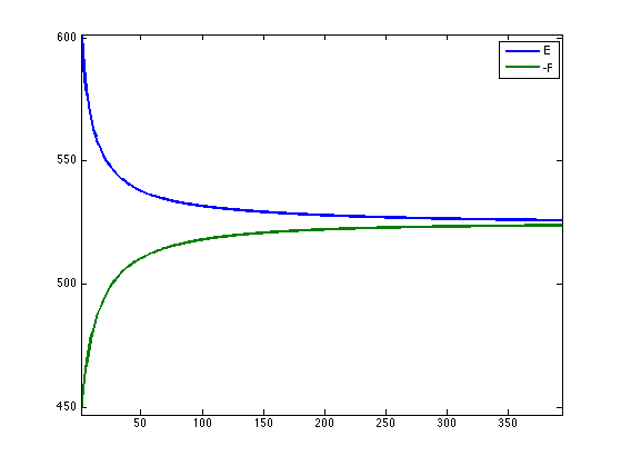
Exercice 1: (check the solution) Perform Chambolle algorithm to solve the ROF problem. Monitor the primal \(E\) and dual \(-F\) energies.

exo1;

Display the denoised image \(x^\star\).

clf;
imageplot(clamp(x));