\[ \newcommand{\NN}{\mathbb{N}} \newcommand{\CC}{\mathbb{C}} \newcommand{\GG}{\mathbb{G}} \newcommand{\LL}{\mathbb{L}} \newcommand{\PP}{\mathbb{P}} \newcommand{\QQ}{\mathbb{Q}} \newcommand{\RR}{\mathbb{R}} \newcommand{\VV}{\mathbb{V}} \newcommand{\ZZ}{\mathbb{Z}} \newcommand{\FF}{\mathbb{F}} \newcommand{\KK}{\mathbb{K}} \newcommand{\UU}{\mathbb{U}} \newcommand{\EE}{\mathbb{E}} \newcommand{\Aa}{\mathcal{A}} \newcommand{\Bb}{\mathcal{B}} \newcommand{\Cc}{\mathcal{C}} \newcommand{\Dd}{\mathcal{D}} \newcommand{\Ee}{\mathcal{E}} \newcommand{\Ff}{\mathcal{F}} \newcommand{\Gg}{\mathcal{G}} \newcommand{\Hh}{\mathcal{H}} \newcommand{\Ii}{\mathcal{I}} \newcommand{\Jj}{\mathcal{J}} \newcommand{\Kk}{\mathcal{K}} \newcommand{\Ll}{\mathcal{L}} \newcommand{\Mm}{\mathcal{M}} \newcommand{\Nn}{\mathcal{N}} \newcommand{\Oo}{\mathcal{O}} \newcommand{\Pp}{\mathcal{P}} \newcommand{\Qq}{\mathcal{Q}} \newcommand{\Rr}{\mathcal{R}} \newcommand{\Ss}{\mathcal{S}} \newcommand{\Tt}{\mathcal{T}} \newcommand{\Uu}{\mathcal{U}} \newcommand{\Vv}{\mathcal{V}} \newcommand{\Ww}{\mathcal{W}} \newcommand{\Xx}{\mathcal{X}} \newcommand{\Yy}{\mathcal{Y}} \newcommand{\Zz}{\mathcal{Z}} \newcommand{\al}{\alpha} \newcommand{\la}{\lambda} \newcommand{\ga}{\gamma} \newcommand{\Ga}{\Gamma} \newcommand{\La}{\Lambda} \newcommand{\Si}{\Sigma} \newcommand{\si}{\sigma} \newcommand{\be}{\beta} \newcommand{\de}{\delta} \newcommand{\De}{\Delta} \renewcommand{\phi}{\varphi} \renewcommand{\th}{\theta} \newcommand{\om}{\omega} \newcommand{\Om}{\Omega} \renewcommand{\epsilon}{\varepsilon} \newcommand{\Calpha}{\mathrm{C}^\al} \newcommand{\Cbeta}{\mathrm{C}^\be} \newcommand{\Cal}{\text{C}^\al} \newcommand{\Cdeux}{\text{C}^{2}} \newcommand{\Cun}{\text{C}^{1}} \newcommand{\Calt}[1]{\text{C}^{#1}} \newcommand{\lun}{\ell^1} \newcommand{\ldeux}{\ell^2} \newcommand{\linf}{\ell^\infty} \newcommand{\ldeuxj}{{\ldeux_j}} \newcommand{\Lun}{\text{\upshape L}^1} \newcommand{\Ldeux}{\text{\upshape L}^2} \newcommand{\Lp}{\text{\upshape L}^p} \newcommand{\Lq}{\text{\upshape L}^q} \newcommand{\Linf}{\text{\upshape L}^\infty} \newcommand{\lzero}{\ell^0} \newcommand{\lp}{\ell^p} \renewcommand{\d}{\ins{d}} \newcommand{\Grad}{\text{Grad}} \newcommand{\grad}{\text{grad}} \renewcommand{\div}{\text{div}} \newcommand{\diag}{\text{diag}} \newcommand{\pd}[2]{ \frac{ \partial #1}{\partial #2} } \newcommand{\pdd}[2]{ \frac{ \partial^2 #1}{\partial #2^2} } \newcommand{\dotp}[2]{\langle #1,\,#2\rangle} \newcommand{\norm}[1]{|\!| #1 |\!|} \newcommand{\normi}[1]{\norm{#1}_{\infty}} \newcommand{\normu}[1]{\norm{#1}_{1}} \newcommand{\normz}[1]{\norm{#1}_{0}} \newcommand{\abs}[1]{\vert #1 \vert} \newcommand{\argmin}{\text{argmin}} \newcommand{\argmax}{\text{argmax}} \newcommand{\uargmin}[1]{\underset{#1}{\argmin}\;} \newcommand{\uargmax}[1]{\underset{#1}{\argmax}\;} \newcommand{\umin}[1]{\underset{#1}{\min}\;} \newcommand{\umax}[1]{\underset{#1}{\max}\;} \newcommand{\pa}[1]{\left( #1 \right)} \newcommand{\choice}[1]{ \left\{ \begin{array}{l} #1 \end{array} \right. } \newcommand{\enscond}[2]{ \left\{ #1 \;:\; #2 \right\} } \newcommand{\qandq}{ \quad \text{and} \quad } \newcommand{\qqandqq}{ \qquad \text{and} \qquad } \newcommand{\qifq}{ \quad \text{if} \quad } \newcommand{\qqifqq}{ \qquad \text{if} \qquad } \newcommand{\qwhereq}{ \quad \text{where} \quad } \newcommand{\qqwhereqq}{ \qquad \text{where} \qquad } \newcommand{\qwithq}{ \quad \text{with} \quad } \newcommand{\qqwithqq}{ \qquad \text{with} \qquad } \newcommand{\qforq}{ \quad \text{for} \quad } \newcommand{\qqforqq}{ \qquad \text{for} \qquad } \newcommand{\qqsinceqq}{ \qquad \text{since} \qquad } \newcommand{\qsinceq}{ \quad \text{since} \quad } \newcommand{\qarrq}{\quad\Longrightarrow\quad} \newcommand{\qqarrqq}{\quad\Longrightarrow\quad} \newcommand{\qiffq}{\quad\Longleftrightarrow\quad} \newcommand{\qqiffqq}{\qquad\Longleftrightarrow\qquad} \newcommand{\qsubjq}{ \quad \text{subject to} \quad } \newcommand{\qqsubjqq}{ \qquad \text{subject to} \qquad } \]

Primal-Dual Proximal Splitting

This tour explores a primal-dual proximal splitting algorithm, with application to imaging problems.

Installing toolboxes and setting up the path.
Convex Optimization with a Primal-Dual Scheme
Inpainting Problem
Total Variation Regularization under Constraints
Primal-dual Total Variation Regularization Algorithm
Inpainting Large Missing Regions

Installing toolboxes and setting up the path.

You need to download the following files: signal toolbox and general toolbox.

You need to unzip these toolboxes in your working directory, so that you have toolbox_signal and toolbox_general in your directory.

For Scilab user: you must replace the Matlab comment '%' by its Scilab counterpart '//'.

Recommandation: You should create a text file named for instance numericaltour.sce (in Scilab) or numericaltour.m (in Matlab) to write all the Scilab/Matlab command you want to execute. Then, simply run exec('numericaltour.sce'); (in Scilab) or numericaltour; (in Matlab) to run the commands.

Execute this line only if you are using Matlab.

getd = @(p)path(p,path); % scilab users must *not* execute this

Then you can add the toolboxes to the path.

getd('toolbox_signal/');
getd('toolbox_general/');

Convex Optimization with a Primal-Dual Scheme

In this tour we use the primal-dual algorithm detailed in:

Antonin Chambolle and Thomas Pock A First-order primal-dual algorithm for convex problems with application to imaging, Journal of Mathematical Imaging and Vision, Volume 40, Number 1 (2011), 120-145

One should note that there exist many other primal-dual schemes.

We consider general optimization problems of the form \[ \umin{f} F(K(f)) + G(f) \] where \(F\) and \(G\) are convex functions and \(K : f \mapsto K(f)\) is a linear operator.

For the primal-dual algorithm to be applicable, one should be able to compute the proximal mapping of \(F\) and \(G\), defined as: \[ \text{Prox}_{\gamma F}(x) = \uargmin{y} \frac{1}{2}\norm{x-y}^2 + \ga F(y) \] (the same definition applies also for \(G\)).

The algorithm reads: \[ g_{k+1} = \text{Prox}_{\sigma F^*}( g_k + \sigma K(\tilde f_k) \] \[ f_{k+1} = \text{Prox}_{\tau G}( f_k-\tau K^*(g_k) ) \] \[ \tilde f_{k+1} = f_{k+1} + \theta (f_{k+1} - f_k) \]

The dual functional is defined as \[ F^*(y) = \umax{x} \dotp{x}{y}-F(x). \] Note that being able to compute the proximal mapping of \(F\) is equivalent to being able to compute the proximal mapping of \(F^*\), thanks to Moreau's identity: \[ x = \text{Prox}_{\tau F^*}(x) + \tau \text{Prox}_{F/\tau}(x/\tau) \]

It can be shown that in the case \(\theta=1\), if \(\sigma \tau \norm{K}^2<1\), then \(f_k\) converges to a minimizer of the original minimization of \(F(K(f)) + G(f)\).

More general primal-dual schemes have been developped, see for instance

L. Condat, A primal-dual splitting method for convex optimization involving Lipschitzian, proximable and linear composite terms, J. Optimization Theory and Applications, 2013, in press.

Inpainting Problem

We consider a linear imaging operator \(\Phi : f \mapsto \Phi(f)\) that maps high resolution images to low dimensional observations. Here we consider a pixel masking operator, that is diagonal over the spacial domain.

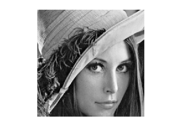
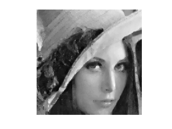
Load an image.

name = 'lena';
n = 256;
f0 = load_image(name);
f0 = rescale(crop(f0,n));

Display it.

clf;
imageplot(f0);

We consider here the inpainting problem. This simply corresponds to a masking operator.

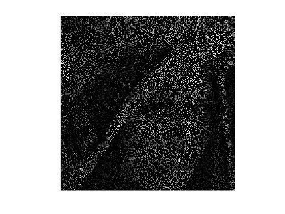
Load a random mask \(\La\).

rho = .8;
Lambda = rand(n,n)>rho;

Masking operator \( \Phi \).

Phi = @(f)f.*Lambda;

Compute the observations \(y=\Phi f_0\).

y = Phi(f0);

Display it.

clf;
imageplot(y);

Total Variation Regularization under Constraints

We want to solve the noiseless inverse problem \(y=\Phi f\) using a total variation regularization: \[ \umin{ y=\Phi f } \norm{\nabla f}_1 \]

This can be recasted as the minimization of \(F(K(f)) + G(f)\) by introducing \[ G(f)=i_H(f), \quad F(u)=\norm{u}_1 \qandq K=\nabla, \] where \(H = \enscond{x}{\Phi(x)=y}\) is an affine space, and \(i_H\) is the indicator function \[ i_H(x) = \choice{ 0 \qifq x \in H, \\ +\infty \qifq x \notin H. } \]

Shorcut for the operators.

K  = @(f)grad(f);
KS = @(u)-div(u);

Shortcut for the TV norm.

Amplitude = @(u)sqrt(sum(u.^2,3));
F = @(u)sum(sum(Amplitude(u)));

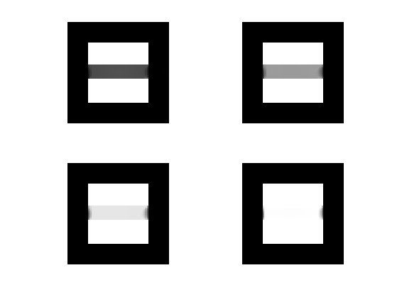
The proximal operator of the vectorial \(\ell^1\) norm reads \[ \text{Prox}_{\lambda F}(u) = \max\pa{0,1-\frac{\la}{\norm{u_k}}} u_k \]

ProxF = @(u,lambda)max(0,1-lambda./repmat(Amplitude(u), [1 1 2])).*u;

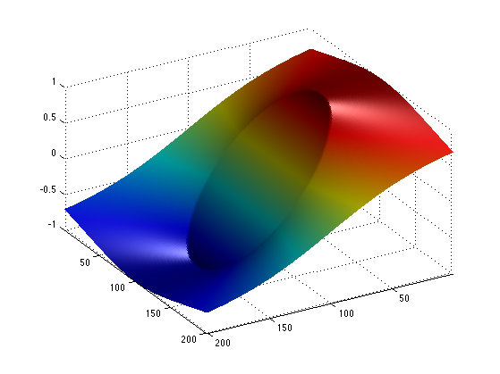
Display the thresholding on the vertical component of the vector.

t = -linspace(-2,2, 201);
[Y,X] = meshgrid(t,t);
U = cat(3,Y,X);
V = ProxF(U,1);
clf;
surf(V(:,:,1));
colormap jet(256);
view(150,40);
axis('tight');
camlight; shading interp;

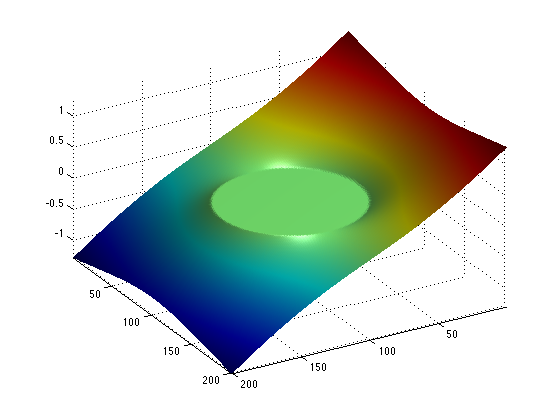
For any 1-homogeneous convex functional, the dual function is the indicator of a convex set. For the \(\ell^1\) norm, it is the indicator of the \(\ell^\infty\) ball \[ F^* = i_{\norm{\cdot}_\infty \leq 1} \qwhereq \norm{u}_\infty = \umax{i} \norm{u_i}. \]

The proximal operator of the dual function is hence a projector (and it does not depend on \(\sigma\) ) \[ \text{Prox}_{\sigma F^*}(u) = \text{Proj}_{\norm{\cdot}_\infty \leq 1}(u). \]

A simple way to compute the proximal operator of the dual function \(F^*\), we make use of Moreau's identity: \[ x = \text{Prox}_{\tau F^*}(x) + \tau \text{Prox}_{F/\tau}(x/\tau) \]

ProxFS = @(y,sigma)y-sigma*ProxF(y/sigma,1/sigma);

Display this dual proximal on the vertical component of the vector.

V = ProxFS(U,1);
clf;
surf(V(:,:,1));
colormap jet(256);
view(150,40);
axis('tight');
camlight; shading interp;

The proximal operator of \(G = i_H\) is the projector on \(H\). In our case, since \(\Phi\) is a diagonal so that the projection is simple to compute \[ \text{Prox}_{\tau G}(f) = \text{Proj}_{H}(f) = f + \Phi(y - \Phi(f)) \]

ProxG = @(f,tau)f + Phi(y - Phi(f));

Primal-dual Total Variation Regularization Algorithm

Now we can apply the primal dual scheme to the TV regularization problem.

We set parameters for the algorithm. Note that in our case, \(L=\norm{K}^2=8\). One should has \(L \sigma \tau < 1\).

L = 8;
sigma = 10;
tau = .9/(L*sigma);
theta = 1;

Initialization, here f stands for the current iterate \(f_k\), g for \(g_k\) and f1 for \(\tilde f_k\).

f = y;
g = K(y)*0;
f1 = f;

Example of one iterations.

fold = f;
g = ProxFS( g+sigma*K(f1), sigma);
f = ProxG(  f-tau*KS(g), tau);
f1 = f + theta * (f-fold);

Exercice 1: (check the solution) Implement the primal-dual algorithm. Monitor the evolution of the TV energy \(F(K(f_k))\) during the iterations. Note that one always has \( f_k \in H \) so that the iterates satisfies the constraints.

exo1;

Display inpainted image.

clf;
imageplot(f);

Exercice 2: (check the solution) Use the primal dual scheme to perform regularization in the presence of noise \[ \umin{\norm{y-\Phi(f)} \leq \epsilon} \norm{\nabla f}_1. \]

exo2;

Inpainting Large Missing Regions

It is possible to consider a more challening problem of inpainting large missing regions.

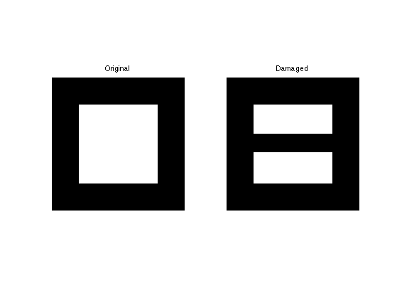
To emphasis the effect of the TV functional, we use a simple geometric image.

n = 64;
name = 'square';
f0 = load_image(name,n);

We remove the central part of the image.

a = 4;
Lambda = ones(n);
Lambda(end/2-a:end/2+a,:) = 0;
Phi = @(f)f.*Lambda;

Display.

clf;
imageplot(f0, 'Original', 1,2,1);
imageplot(Phi(f0), 'Damaged', 1,2,2);

Exercice 3: (check the solution) Display the evolution of the inpainting process.

exo3;