\[ \newcommand{\NN}{\mathbb{N}} \newcommand{\CC}{\mathbb{C}} \newcommand{\GG}{\mathbb{G}} \newcommand{\LL}{\mathbb{L}} \newcommand{\PP}{\mathbb{P}} \newcommand{\QQ}{\mathbb{Q}} \newcommand{\RR}{\mathbb{R}} \newcommand{\VV}{\mathbb{V}} \newcommand{\ZZ}{\mathbb{Z}} \newcommand{\FF}{\mathbb{F}} \newcommand{\KK}{\mathbb{K}} \newcommand{\UU}{\mathbb{U}} \newcommand{\EE}{\mathbb{E}} \newcommand{\Aa}{\mathcal{A}} \newcommand{\Bb}{\mathcal{B}} \newcommand{\Cc}{\mathcal{C}} \newcommand{\Dd}{\mathcal{D}} \newcommand{\Ee}{\mathcal{E}} \newcommand{\Ff}{\mathcal{F}} \newcommand{\Gg}{\mathcal{G}} \newcommand{\Hh}{\mathcal{H}} \newcommand{\Ii}{\mathcal{I}} \newcommand{\Jj}{\mathcal{J}} \newcommand{\Kk}{\mathcal{K}} \newcommand{\Ll}{\mathcal{L}} \newcommand{\Mm}{\mathcal{M}} \newcommand{\Nn}{\mathcal{N}} \newcommand{\Oo}{\mathcal{O}} \newcommand{\Pp}{\mathcal{P}} \newcommand{\Qq}{\mathcal{Q}} \newcommand{\Rr}{\mathcal{R}} \newcommand{\Ss}{\mathcal{S}} \newcommand{\Tt}{\mathcal{T}} \newcommand{\Uu}{\mathcal{U}} \newcommand{\Vv}{\mathcal{V}} \newcommand{\Ww}{\mathcal{W}} \newcommand{\Xx}{\mathcal{X}} \newcommand{\Yy}{\mathcal{Y}} \newcommand{\Zz}{\mathcal{Z}} \newcommand{\al}{\alpha} \newcommand{\la}{\lambda} \newcommand{\ga}{\gamma} \newcommand{\Ga}{\Gamma} \newcommand{\La}{\Lambda} \newcommand{\Si}{\Sigma} \newcommand{\si}{\sigma} \newcommand{\be}{\beta} \newcommand{\de}{\delta} \newcommand{\De}{\Delta} \renewcommand{\phi}{\varphi} \renewcommand{\th}{\theta} \newcommand{\om}{\omega} \newcommand{\Om}{\Omega} \renewcommand{\epsilon}{\varepsilon} \newcommand{\Calpha}{\mathrm{C}^\al} \newcommand{\Cbeta}{\mathrm{C}^\be} \newcommand{\Cal}{\text{C}^\al} \newcommand{\Cdeux}{\text{C}^{2}} \newcommand{\Cun}{\text{C}^{1}} \newcommand{\Calt}[1]{\text{C}^{#1}} \newcommand{\lun}{\ell^1} \newcommand{\ldeux}{\ell^2} \newcommand{\linf}{\ell^\infty} \newcommand{\ldeuxj}{{\ldeux_j}} \newcommand{\Lun}{\text{\upshape L}^1} \newcommand{\Ldeux}{\text{\upshape L}^2} \newcommand{\Lp}{\text{\upshape L}^p} \newcommand{\Lq}{\text{\upshape L}^q} \newcommand{\Linf}{\text{\upshape L}^\infty} \newcommand{\lzero}{\ell^0} \newcommand{\lp}{\ell^p} \renewcommand{\d}{\ins{d}} \newcommand{\Grad}{\text{Grad}} \newcommand{\grad}{\text{grad}} \renewcommand{\div}{\text{div}} \newcommand{\diag}{\text{diag}} \newcommand{\pd}[2]{ \frac{ \partial #1}{\partial #2} } \newcommand{\pdd}[2]{ \frac{ \partial^2 #1}{\partial #2^2} } \newcommand{\dotp}[2]{\langle #1,\,#2\rangle} \newcommand{\norm}[1]{|\!| #1 |\!|} \newcommand{\normi}[1]{\norm{#1}_{\infty}} \newcommand{\normu}[1]{\norm{#1}_{1}} \newcommand{\normz}[1]{\norm{#1}_{0}} \newcommand{\abs}[1]{\vert #1 \vert} \newcommand{\argmin}{\text{argmin}} \newcommand{\argmax}{\text{argmax}} \newcommand{\uargmin}[1]{\underset{#1}{\argmin}\;} \newcommand{\uargmax}[1]{\underset{#1}{\argmax}\;} \newcommand{\umin}[1]{\underset{#1}{\min}\;} \newcommand{\umax}[1]{\underset{#1}{\max}\;} \newcommand{\pa}[1]{\left( #1 \right)} \newcommand{\choice}[1]{ \left\{ \begin{array}{l} #1 \end{array} \right. } \newcommand{\enscond}[2]{ \left\{ #1 \;:\; #2 \right\} } \newcommand{\qandq}{ \quad \text{and} \quad } \newcommand{\qqandqq}{ \qquad \text{and} \qquad } \newcommand{\qifq}{ \quad \text{if} \quad } \newcommand{\qqifqq}{ \qquad \text{if} \qquad } \newcommand{\qwhereq}{ \quad \text{where} \quad } \newcommand{\qqwhereqq}{ \qquad \text{where} \qquad } \newcommand{\qwithq}{ \quad \text{with} \quad } \newcommand{\qqwithqq}{ \qquad \text{with} \qquad } \newcommand{\qforq}{ \quad \text{for} \quad } \newcommand{\qqforqq}{ \qquad \text{for} \qquad } \newcommand{\qqsinceqq}{ \qquad \text{since} \qquad } \newcommand{\qsinceq}{ \quad \text{since} \quad } \newcommand{\qarrq}{\quad\Longrightarrow\quad} \newcommand{\qqarrqq}{\quad\Longrightarrow\quad} \newcommand{\qiffq}{\quad\Longleftrightarrow\quad} \newcommand{\qqiffqq}{\qquad\Longleftrightarrow\qquad} \newcommand{\qsubjq}{ \quad \text{subject to} \quad } \newcommand{\qqsubjqq}{ \qquad \text{subject to} \qquad } \]

Forward-Backward Proximal Splitting

This numerical tour presents the Forward-Backward (FB) algorithm to minimize the sum of a smooth and a simple function. It shows an application to sparse-spikes deconvolution.

Installing toolboxes and setting up the path.
Bibliography
Forward-Backward Algorithm
Sparse Regularization of Inverse Problems
Signal Deconvolution Problem on Synthetic Sparse Data
Sparse-Spikes Deconvolution
Over-relaxed Forward-Backward
FISTA Accelerated Algorithm

Installing toolboxes and setting up the path.

You need to download the following files: signal toolbox and general toolbox.

You need to unzip these toolboxes in your working directory, so that you have toolbox_signal and toolbox_general in your directory.

For Scilab user: you must replace the Matlab comment '%' by its Scilab counterpart '//'.

Recommandation: You should create a text file named for instance numericaltour.sce (in Scilab) or numericaltour.m (in Matlab) to write all the Scilab/Matlab command you want to execute. Then, simply run exec('numericaltour.sce'); (in Scilab) or numericaltour; (in Matlab) to run the commands.

Execute this line only if you are using Matlab.

getd = @(p)path(p,path); % scilab users must *not* execute this

Then you can add the toolboxes to the path.

getd('toolbox_signal/');
getd('toolbox_general/');

Bibliography

Excellent review papers on proximal splitting algorithms include:

Amir Beck and Marc Teboulle, Gradient-Based Algorithms with Applications to Signal Recovery Problems, in "Convex Optimization in Signal Processing and Communications". Editors: Yonina Eldar and Daniel Palomar. Cambridge university press.

P. L. Combettes and J.-C. Pesquet, Proximal splitting methods in signal processing, in: Fixed-Point Algorithms for Inverse Problems in Science and Engineering, (H. H. Bauschke, R. S. Burachik, P. L. Combettes, V. Elser, D. R. Luke, and H. Wolkowicz, Editors), pp. 185-212. Springer, New York, 2011.

Forward-Backward Algorithm

We consider the problem of minimizing the sum of two functions \[ E^\star \umin{x \in \RR^N} E(x) = f(x) + g(x). \]

We assume that \(f\) is a \(C^1\) function with \(L\)-Lipschitz gradient, which means that \[ \forall (x,y) \in \RR^N \times \RR^N, \quad \norm{\nabla f(x) - \nabla f(y)} \leq L \norm{x-y}. \]

We also assume that \(g\) is "simple", in the sense that one can compute in closed form the so-called proximal mapping, which is defined as \[ \text{prox}_{\ga g}(x) = \uargmin{y \in \RR^N} \frac{1}{2}\norm{x-y}^2 + \ga g(y). \] for any \(\ga > 0\).

The FB algorithm reads, after initilizing \(x^{(0)} \in \RR^N\), \[ x^{(\ell+1)} = \text{prox}_{\ga g}\pa{ x^{(\ell)} - \ga \nabla f( x^{(\ell)} ) }. \]

If \(0 < \ga < 2/L\), then this scheme converges to a minimizer of \(f+g\).

Sparse Regularization of Inverse Problems

We consider a linear inverse problem \[ y = \Phi x_0 + w \in \RR^P\] where \(x_0 \in \RR^N\) is the (unknown) signal to recover, \(w \in \RR^P\) is a noise vector, and \(\Phi \in \RR^{P \times N}\) models the acquisition device.

To recover an approximation of the signal \(x_0\), we use the Basis Pursuit denoising method, that use the \(\ell^1\) norm as a sparsity enforcing penalty \[ \umin{x \in \RR^N} \frac{1}{2} \norm{y-\Phi x}^2 + \la \norm{x}_1, \] where the \(\ell^1\) norm is defined as \[ \norm{x}_1 = \sum_i \abs{x_i}. \]

The parameter \(\la\) should be set in accordance to the noise level \(\norm{w}\).

This minimization problem can be cast in the form of minimizing \(f+g\) where \[ f(x) = \frac{1}{2} \norm{y-\Phi x}^2 \qandq g(x) = \la \norm{x}_1. \]

\(f\) is a smooth function, which satisfies \[ \nabla f(x) = \Phi^* (\Phi x - y), \] it has a \(L\)-Lipschitz gradient with \[ L = \norm{ \Phi^* \Phi }. \]

The \(\ell^1\)-norm is "simple", because its proximal operator is a soft thresholding: \[ \text{prox}_{\ga g}(x)_k = \max\pa{ 0, 1 - \frac{\la \ga}{\abs{x_k}} } x_k. \]

Signal Deconvolution Problem on Synthetic Sparse Data

A simple linearized model of seismic acquisition consider a linear operator which is a filtering \[ \Phi x = \phi \star x \]

Dimension of the problem.

N = 1024;

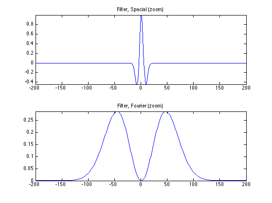
We load a seismic filter \(\phi\), which is a second derivative of a Gaussian.

Width of the filter.

s = 5;

Second derivative of Gaussian.

t = (-N/2:N/2-1)';
h = (1-t.^2/s^2).*exp( -(t.^2)/(2*s^2) );
h = h-mean(h);

Define the operator \(\Phi\).

h1 = fftshift(h); % Recenter the filter for fft use.
Phi = @(u)real(ifft(fft(h1).*fft(u)));

Display the filter and its Fourier transform.

% Fourier transform (normalized)
hf = real(fftshift(fft(h1))) / sqrt(N);
% display
q = 200;
clf;
subplot(2,1,1);
plot(-N/2+1:N/2, h);
axis([-q q min(h) max(h)]);
title('Filter, Spacial (zoom)');
subplot(2,1,2);
plot(-N/2+1:N/2, hf);
axis([-q q 0 max(hf)]);
title('Filter, Fourier (zoom)');

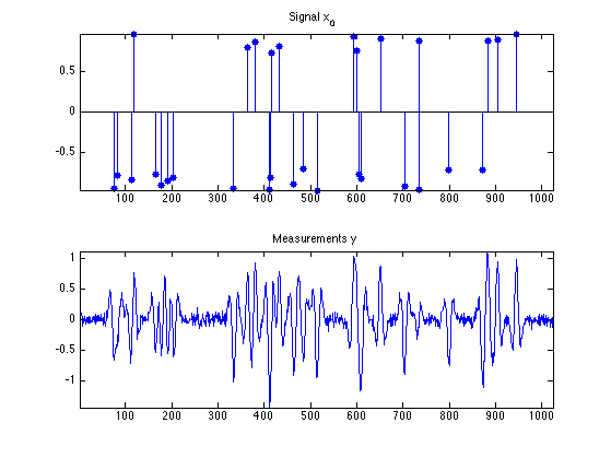
We generate a synthetic sparse signal \(x_0\), with only a small number of non zero coefficients.

Number of Diracs of the signal.

s = round(N*.03);

Set the seed-number (for reproductibility).

rand('state', 1);
randn('state', 1);

Location of the diracs.

sel = randperm(N); sel = sel(1:s);

Signal \(x_0\).

x0 = zeros(N,1); x0(sel) = 1;
x0 = x0 .* sign(randn(N,1)) .* (1-.3*rand(N,1));

Noise level.

sigma = .06;

Compute the measurements \(y=\Phi x_0 + w\) where \(w\) is a realization of a Gaussian white noise of variance \(\si^2\).

y = Phi(x0) + sigma*randn(N,1);

Display signals and measurements.

clf; ms = 20;
subplot(2,1,1);
u = x0; u(x0==0) = NaN;
stem(u, 'b.', 'MarkerSize', ms); axis('tight');
title('Signal x_0');
subplot(2,1,2);
plot(y); axis('tight');
title('Measurements y');

Sparse-Spikes Deconvolution

We now implement the FB algorithm for the sparse spikes problem.

Regularization strenght \(\la\).

lambda = 1;

Define the proximity operator of \(\ga g\).

proxg = @(x,gamma)perform_thresholding(x, lambda*gamma, 'soft');

Define the gradient operator of \(f\)

gradf = @(x)Phi(Phi(x)-y);

Define the Lipschitz constant of \(f\).

L = max(abs(fft(h)))^2;

Gradient step size \(\ga\), should be smaller than \(2/L\).

gamma = 1.95 / L;

Initialization \(x^{(0)}\).

x = y;

Perform one step of FB.

x = proxg( x - gamma*gradf(x), gamma );

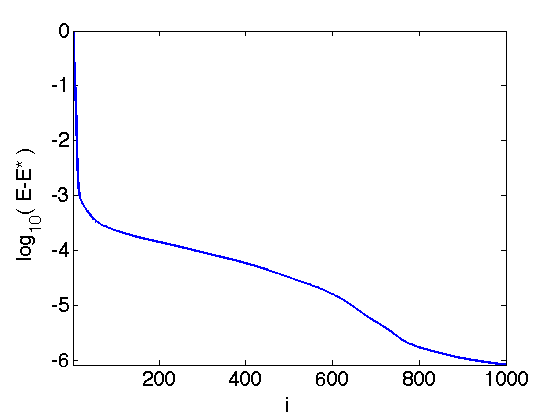
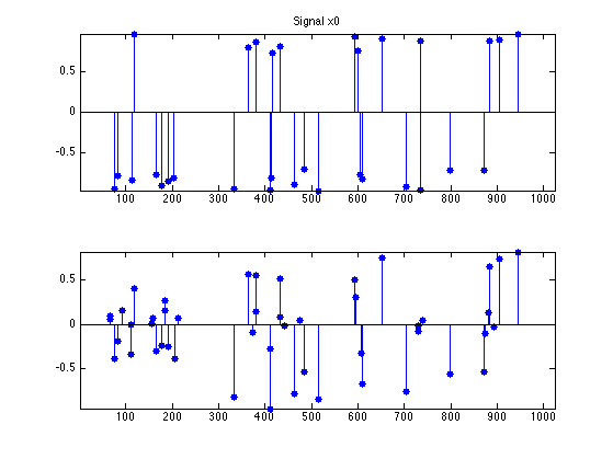
Exercice 1: (check the solution) Compute the solution of L1 deconvolution. Keep track of the degay of the energy \(E=f+g\).

exo1;

Display the result.

clf;
subplot(2,1,1);
u = x0; u(x0==0) = NaN;
stem(u, 'b.', 'MarkerSize', ms); axis('tight');
title(['Signal x0']);
subplot(2,1,2);
u = x; u(x==0) = NaN;
stem(u, 'b.', 'MarkerSize', ms); axis('tight');

Over-relaxed Forward-Backward

It is possible to introduce a relaxation parameter \(-1 < \mu < 1\) to average the current iterate of the FB with the previous one. In this case, one must set the descent paramter to \[ \ga=\frac{1}{L}. \]

gamma = 1/L;

The algorithm initializes \(z^{(1)}=x^{(0)} \in \RR^N\), and then it computes \[ x^{(\ell)} = \text{prox}_{\ga g}\pa{ z^{(\ell)} - \ga \nabla f( z^{(\ell)} ) }. \] \[ z^{(\ell+1)} = x^{(\ell)} + \mu \pa{ x^{(\ell)} - x^{(\ell-1)} } \]

The regime \(-1<\mu <0\) corresponds to under-relaxation. Setting \(\mu=0\), one recovers the unrelaxed Forward-Backward. Setting \(0 < \mu < 1\) creates over-relaxation.

Note that convergence of the iterates \(x^{(\ell)}\) is only guaranteed for \( -1 < \mu < 1/2 \), and that one can only prove convergence of \( E(x^{(\ell)}) \) toward \(E^\star\) in case \( \mu \in [1/2,1[ \).

For a in-depth analysis of this scheme, see the book:

H.H. Bauschke and P.L. Combettes, Convex Analysis and Monotone Operator Theory in Hilbert Spaces Springer-Verlag (2011)

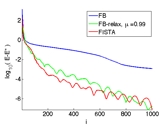
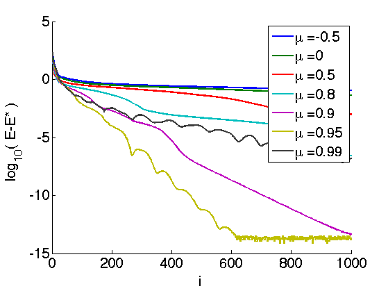
Exercice 2: (check the solution) Impement the relaxed FB algorithm and display its convergence rate for several values of \(\mu\).

exo2;

FISTA Accelerated Algorithm

It is possible to use an adaptive relaxation parameter \(\mu = \mu^{(\ell)}\) that changes from iteration to iteration.

This strategy is used in the Fast Iterative Soft Thresholding (FISTA) algorithm introduced in:

Amir Beck and Marc Teboulle, A Fast Iterative Shrinkage-Thresholding Algorithm for Linear Inverse Problems, SIAM Journal on Imaging Sciences 2 (2009), no. 1, 183--202.

In this algorithm, the relaxation parameters \(\mu^{(\ell)}\) are automatically set and tend to the limit value \[ \mu^{(\ell)} \overset{\ell \rightarrow +\infty}{\longrightarrow} 1 . \]

The step size should be set to: \[ \ga = \frac{1}{L}. \]

gamma = 1/L;

The algorithm initializes \(z^{(1)}=x^{(0)} \in \RR^N\), and \(t^{(1)}=1\) and then it computes \[ x^{(\ell)} = \text{prox}_{\ga g}\pa{ z^{(\ell)} - \ga \nabla f( z^{(\ell)} ) }. \] \[ t^{(\ell+1)} = \frac{ 1 + \sqrt{1+4(t^{(\ell)})^2} }{2} \qandq \mu^{(\ell+1)} = \frac{t^{(\ell)}-1}{ t^{(\ell+1)} } \] \[ z^{(\ell+1)} = x^{(\ell+1)} + \mu^{(\ell+1)} \pa{ x^{(\ell)} - x^{(\ell-1)} } \]

For this scheme, one cannot prove convergence of the iterates, but one can prove that it reaches an optimal convergence rate of the iterates, namely \[ E(f^{(\ell)}) - E^\star = O(1/\ell^2) \] while the convergence rate for the usual FB is only \(O(1/\ell)\).

Exercice 3: (check the solution) Compute the solution of L1 deconvolution using FISTA. Keep track of the degay of the energy \(E = f+g\).

exo3;