\[ \newcommand{\NN}{\mathbb{N}} \newcommand{\CC}{\mathbb{C}} \newcommand{\GG}{\mathbb{G}} \newcommand{\LL}{\mathbb{L}} \newcommand{\PP}{\mathbb{P}} \newcommand{\QQ}{\mathbb{Q}} \newcommand{\RR}{\mathbb{R}} \newcommand{\VV}{\mathbb{V}} \newcommand{\ZZ}{\mathbb{Z}} \newcommand{\FF}{\mathbb{F}} \newcommand{\KK}{\mathbb{K}} \newcommand{\UU}{\mathbb{U}} \newcommand{\EE}{\mathbb{E}} \newcommand{\Aa}{\mathcal{A}} \newcommand{\Bb}{\mathcal{B}} \newcommand{\Cc}{\mathcal{C}} \newcommand{\Dd}{\mathcal{D}} \newcommand{\Ee}{\mathcal{E}} \newcommand{\Ff}{\mathcal{F}} \newcommand{\Gg}{\mathcal{G}} \newcommand{\Hh}{\mathcal{H}} \newcommand{\Ii}{\mathcal{I}} \newcommand{\Jj}{\mathcal{J}} \newcommand{\Kk}{\mathcal{K}} \newcommand{\Ll}{\mathcal{L}} \newcommand{\Mm}{\mathcal{M}} \newcommand{\Nn}{\mathcal{N}} \newcommand{\Oo}{\mathcal{O}} \newcommand{\Pp}{\mathcal{P}} \newcommand{\Qq}{\mathcal{Q}} \newcommand{\Rr}{\mathcal{R}} \newcommand{\Ss}{\mathcal{S}} \newcommand{\Tt}{\mathcal{T}} \newcommand{\Uu}{\mathcal{U}} \newcommand{\Vv}{\mathcal{V}} \newcommand{\Ww}{\mathcal{W}} \newcommand{\Xx}{\mathcal{X}} \newcommand{\Yy}{\mathcal{Y}} \newcommand{\Zz}{\mathcal{Z}} \newcommand{\al}{\alpha} \newcommand{\la}{\lambda} \newcommand{\ga}{\gamma} \newcommand{\Ga}{\Gamma} \newcommand{\La}{\Lambda} \newcommand{\Si}{\Sigma} \newcommand{\si}{\sigma} \newcommand{\be}{\beta} \newcommand{\de}{\delta} \newcommand{\De}{\Delta} \renewcommand{\phi}{\varphi} \renewcommand{\th}{\theta} \newcommand{\om}{\omega} \newcommand{\Om}{\Omega} \renewcommand{\epsilon}{\varepsilon} \newcommand{\Calpha}{\mathrm{C}^\al} \newcommand{\Cbeta}{\mathrm{C}^\be} \newcommand{\Cal}{\text{C}^\al} \newcommand{\Cdeux}{\text{C}^{2}} \newcommand{\Cun}{\text{C}^{1}} \newcommand{\Calt}[1]{\text{C}^{#1}} \newcommand{\lun}{\ell^1} \newcommand{\ldeux}{\ell^2} \newcommand{\linf}{\ell^\infty} \newcommand{\ldeuxj}{{\ldeux_j}} \newcommand{\Lun}{\text{\upshape L}^1} \newcommand{\Ldeux}{\text{\upshape L}^2} \newcommand{\Lp}{\text{\upshape L}^p} \newcommand{\Lq}{\text{\upshape L}^q} \newcommand{\Linf}{\text{\upshape L}^\infty} \newcommand{\lzero}{\ell^0} \newcommand{\lp}{\ell^p} \renewcommand{\d}{\ins{d}} \newcommand{\Grad}{\text{Grad}} \newcommand{\grad}{\text{grad}} \renewcommand{\div}{\text{div}} \newcommand{\diag}{\text{diag}} \newcommand{\pd}[2]{ \frac{ \partial #1}{\partial #2} } \newcommand{\pdd}[2]{ \frac{ \partial^2 #1}{\partial #2^2} } \newcommand{\dotp}[2]{\langle #1,\,#2\rangle} \newcommand{\norm}[1]{|\!| #1 |\!|} \newcommand{\normi}[1]{\norm{#1}_{\infty}} \newcommand{\normu}[1]{\norm{#1}_{1}} \newcommand{\normz}[1]{\norm{#1}_{0}} \newcommand{\abs}[1]{\vert #1 \vert} \newcommand{\argmin}{\text{argmin}} \newcommand{\argmax}{\text{argmax}} \newcommand{\uargmin}[1]{\underset{#1}{\argmin}\;} \newcommand{\uargmax}[1]{\underset{#1}{\argmax}\;} \newcommand{\umin}[1]{\underset{#1}{\min}\;} \newcommand{\umax}[1]{\underset{#1}{\max}\;} \newcommand{\pa}[1]{\left( #1 \right)} \newcommand{\choice}[1]{ \left\{ \begin{array}{l} #1 \end{array} \right. } \newcommand{\enscond}[2]{ \left\{ #1 \;:\; #2 \right\} } \newcommand{\qandq}{ \quad \text{and} \quad } \newcommand{\qqandqq}{ \qquad \text{and} \qquad } \newcommand{\qifq}{ \quad \text{if} \quad } \newcommand{\qqifqq}{ \qquad \text{if} \qquad } \newcommand{\qwhereq}{ \quad \text{where} \quad } \newcommand{\qqwhereqq}{ \qquad \text{where} \qquad } \newcommand{\qwithq}{ \quad \text{with} \quad } \newcommand{\qqwithqq}{ \qquad \text{with} \qquad } \newcommand{\qforq}{ \quad \text{for} \quad } \newcommand{\qqforqq}{ \qquad \text{for} \qquad } \newcommand{\qqsinceqq}{ \qquad \text{since} \qquad } \newcommand{\qsinceq}{ \quad \text{since} \quad } \newcommand{\qarrq}{\quad\Longrightarrow\quad} \newcommand{\qqarrqq}{\quad\Longrightarrow\quad} \newcommand{\qiffq}{\quad\Longleftrightarrow\quad} \newcommand{\qqiffqq}{\qquad\Longleftrightarrow\qquad} \newcommand{\qsubjq}{ \quad \text{subject to} \quad } \newcommand{\qqsubjqq}{ \qquad \text{subject to} \qquad } \]

Mesh Deformation

This tour explores deformation of 2D mesh using Laplacian interpolation. The dense deformation field is obtained from a sparse set of displaced anchor point by computing harmonic interpolation.

Contents

• Installing toolboxes and setting up the path.
• Mesh Creation
• Boundary Modification
• Non-linear Deformation
• Bi-Laplacian Deformation

Installing toolboxes and setting up the path.

You need to download the following files: signal toolbox, general toolbox and graph toolbox.

You need to unzip these toolboxes in your working directory, so that you have toolbox_signal, toolbox_general and toolbox_graph in your directory.

For Scilab user: you must replace the Matlab comment '%' by its Scilab counterpart '//'.

Recommandation: You should create a text file named for instance numericaltour.sce (in Scilab) or numericaltour.m (in Matlab) to write all the Scilab/Matlab command you want to execute. Then, simply run exec('numericaltour.sce'); (in Scilab) or numericaltour; (in Matlab) to run the commands.

Execute this line only if you are using Matlab.

getd = @(p)path(p,path); % scilab users must *not* execute this

Then you can add the toolboxes to the path.

getd('toolbox_signal/');
getd('toolbox_general/');
getd('toolbox_graph/');

Mesh Creation

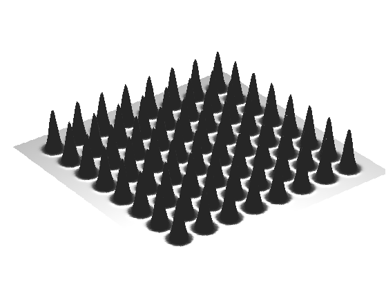
We create a simple mesh with fine scale details.

We generate point on a square.

p = 150;
[Y,X] = meshgrid(linspace(-1,1,p),linspace(-1,1,p));
vertex0 = [X(:)'; Y(:)'; zeros(1,p^2)];
n = size(vertex0,2);

We generate a triangulation of a square.

I = reshape(1:p^2,p,p);
a = I(1:p-1,1:p-1); b = I(2:p,1:p-1); c = I(1:p-1,2:p);
d = I(2:p,1:p-1); e = I(2:p,2:p); f = I(1:p-1,2:p);
faces = cat(1, [a(:) b(:) c(:)], [d(:) e(:) f(:)])';

Width and height of the bumps.

sigma = .03;
h = .35;
q = 8;

Elevate the surface using bumps.

t = linspace(-1,1,q+2); t([1 length(t)]) = [];
vertex = vertex0;
for i=1:q
    for j=1:q
        d = (X(:)'-t(i)).^2 + (Y(:)'-t(j)).^2;
        vertex(3,:) = vertex(3,:) + h * exp( -d/(2*sigma^2)  );
    end
end

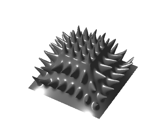
Display the surface.

clf;
plot_mesh(vertex,faces);
view(3);

Compute its geometric (cotan) Laplacian

W = sparse(n,n);
for i=1:3
   i1 = mod(i-1,3)+1;
   i2 = mod(i  ,3)+1;
   i3 = mod(i+1,3)+1;
   pp = vertex(:,faces(i2,:)) - vertex(:,faces(i1,:));
   qq = vertex(:,faces(i3,:)) - vertex(:,faces(i1,:));
   % normalize the vectors
   pp = pp ./ repmat( sqrt(sum(pp.^2,1)), [3 1] );
   qq = qq ./ repmat( sqrt(sum(qq.^2,1)), [3 1] );
   % compute angles
   ang = acos(sum(pp.*qq,1));
   u = cot(ang);
   u = clamp(u, 0.01,100);
   W = W + sparse(faces(i2,:),faces(i3,:),u,n,n);
   W = W + sparse(faces(i3,:),faces(i2,:),u,n,n);
end

Compute the symmetric Laplacian matrix.

d = full( sum(W,1) );
D = spdiags(d(:), 0, n,n);
L = D - W;

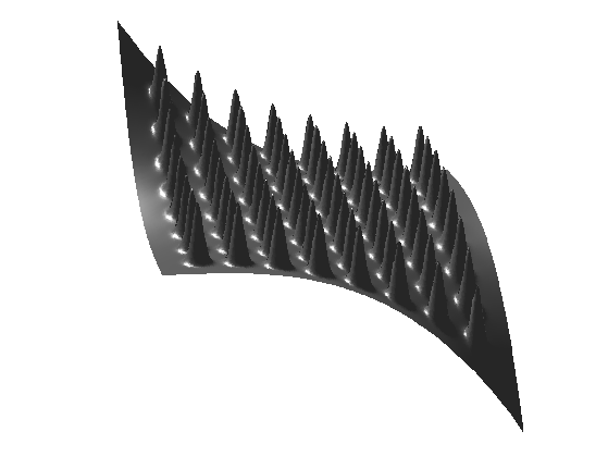
Boundary Modification

We modify the domain by modifying its boundary.

Select boundary indexes.

I = find( abs(X(:))==1 | abs(Y(:))==1 );

Compute the deformation field (zeros outsize the handle, proportional to the normal otherwise).

Delta0 = zeros(3,n);
d = ( vertex(1,I) + vertex(2,I) ) / 2;
Delta0(3,I) = sign(d) .* abs(d).^3;

Modify the Laplacian to take into account the fixed handles.

L1 = L;
L1(I,:) = 0;
L1(I + (I-1)*n) = 1;

Compute the full deformation by solving for Laplacian=0 on each coordinate.

Delta = ( L1 \ Delta0' )';

Compute the deformed mesh.

vertex1 = vertex+Delta;

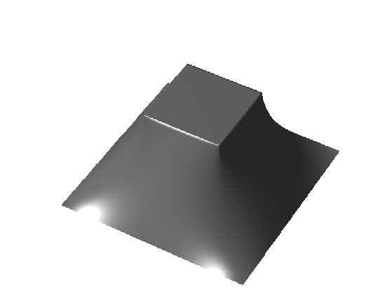
Display it.

clf;
plot_mesh(vertex1,faces);
view(-100,15);

Exercice 1: (check the solution) Perform a more complicated deformation of the boundary.

exo1;

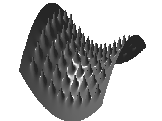
Exercice 2: (check the solution) Move both the inside and the boundary.

exo2;

Exercice 3: (check the solution) Apply the mesh deformation method to a real mesh, with both large scale and fine scale details.

exo3;

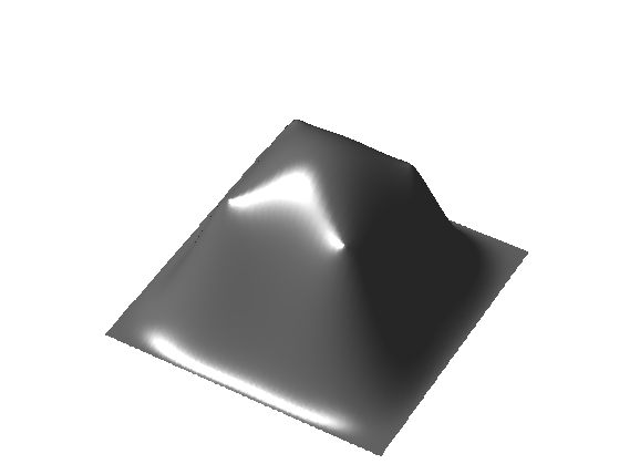
Non-linear Deformation

Linear methods give poor results for large deformation.

It is possible to obtain better result by applying the linear deformation only to a low pass version of the mesh (coarse scale modifications). The remaining details are then added in the direction of the normal, in a local frame that is rotated to match the deformation of the coarse surface.

Exercice 4: (check the solution) Apply the deformation to the coarse mesh vertex0 to obtain vertex1. Important: you need to compute and use the cotan Laplacian of the coarse mesh, not of the original mesh!

exo4;

Compute the residual vector contribution along the normal (which is vertical).

normal = compute_normal(vertex0,faces);
d = repmat( sum(normal .* (vertex-vertex0)), [3 1]);

Exercice 5: (check the solution) Add the normal contribution d.*normal to vertex1, but after replacing the normal of vertex0 by the normal of vertex1.

exo5;

Exercice 6: (check the solution) Try on other surfaces. How can you compute vertex0 for an arbitrary surface ?

exo6;

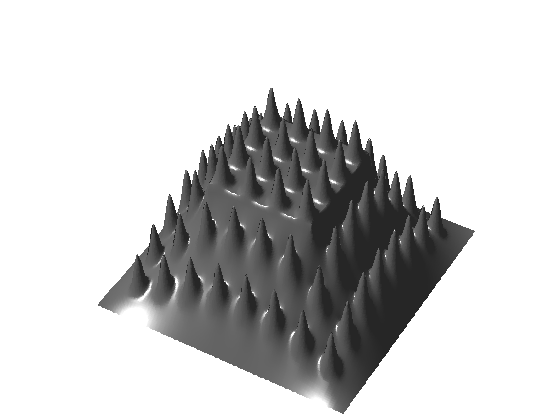
Bi-Laplacian Deformation

To take into account the bending of the surface, one can use higher order derivative to interpolate the deformation field.

The bi-laplacian LL corresponds to 4th order derivatives. It is the square of the Laplacian LL=L*L.

Exercice 7: (check the solution) Compute the bi-laplacian deformation of the coarse shape vertex0 by using LL instead of L. What do you observe ?

exo7;

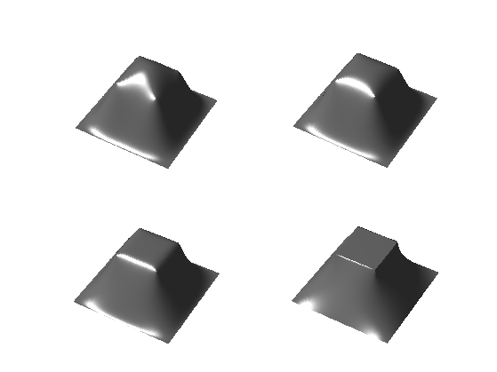
Exercice 8: (check the solution) Compute the deformation obtained by moving from the Laplacian to the bi-laplacian, i.e. with t*L+(1-t)*LL for varying t.

exo8;

Exercice 9: (check the solution) Apply the full model (Laplacian, bi-Laplacian and non-linear deformation) to the deformation of a complicated mesh.

exo9;

Copyright (c) 2010 Gabriel Peyre