\[
\newcommand{\NN}{\mathbb{N}}
\newcommand{\CC}{\mathbb{C}}
\newcommand{\GG}{\mathbb{G}}
\newcommand{\LL}{\mathbb{L}}
\newcommand{\PP}{\mathbb{P}}
\newcommand{\QQ}{\mathbb{Q}}
\newcommand{\RR}{\mathbb{R}}
\newcommand{\VV}{\mathbb{V}}
\newcommand{\ZZ}{\mathbb{Z}}
\newcommand{\FF}{\mathbb{F}}
\newcommand{\KK}{\mathbb{K}}
\newcommand{\UU}{\mathbb{U}}
\newcommand{\EE}{\mathbb{E}}
\newcommand{\Aa}{\mathcal{A}}
\newcommand{\Bb}{\mathcal{B}}
\newcommand{\Cc}{\mathcal{C}}
\newcommand{\Dd}{\mathcal{D}}
\newcommand{\Ee}{\mathcal{E}}
\newcommand{\Ff}{\mathcal{F}}
\newcommand{\Gg}{\mathcal{G}}
\newcommand{\Hh}{\mathcal{H}}
\newcommand{\Ii}{\mathcal{I}}
\newcommand{\Jj}{\mathcal{J}}
\newcommand{\Kk}{\mathcal{K}}
\newcommand{\Ll}{\mathcal{L}}
\newcommand{\Mm}{\mathcal{M}}
\newcommand{\Nn}{\mathcal{N}}
\newcommand{\Oo}{\mathcal{O}}
\newcommand{\Pp}{\mathcal{P}}
\newcommand{\Qq}{\mathcal{Q}}
\newcommand{\Rr}{\mathcal{R}}
\newcommand{\Ss}{\mathcal{S}}
\newcommand{\Tt}{\mathcal{T}}
\newcommand{\Uu}{\mathcal{U}}
\newcommand{\Vv}{\mathcal{V}}
\newcommand{\Ww}{\mathcal{W}}
\newcommand{\Xx}{\mathcal{X}}
\newcommand{\Yy}{\mathcal{Y}}
\newcommand{\Zz}{\mathcal{Z}}
\newcommand{\al}{\alpha}
\newcommand{\la}{\lambda}
\newcommand{\ga}{\gamma}
\newcommand{\Ga}{\Gamma}
\newcommand{\La}{\Lambda}
\newcommand{\Si}{\Sigma}
\newcommand{\si}{\sigma}
\newcommand{\be}{\beta}
\newcommand{\de}{\delta}
\newcommand{\De}{\Delta}
\renewcommand{\phi}{\varphi}
\renewcommand{\th}{\theta}
\newcommand{\om}{\omega}
\newcommand{\Om}{\Omega}
\renewcommand{\epsilon}{\varepsilon}
\newcommand{\Calpha}{\mathrm{C}^\al}
\newcommand{\Cbeta}{\mathrm{C}^\be}
\newcommand{\Cal}{\text{C}^\al}
\newcommand{\Cdeux}{\text{C}^{2}}
\newcommand{\Cun}{\text{C}^{1}}
\newcommand{\Calt}[1]{\text{C}^{#1}}
\newcommand{\lun}{\ell^1}
\newcommand{\ldeux}{\ell^2}
\newcommand{\linf}{\ell^\infty}
\newcommand{\ldeuxj}{{\ldeux_j}}
\newcommand{\Lun}{\text{\upshape L}^1}
\newcommand{\Ldeux}{\text{\upshape L}^2}
\newcommand{\Lp}{\text{\upshape L}^p}
\newcommand{\Lq}{\text{\upshape L}^q}
\newcommand{\Linf}{\text{\upshape L}^\infty}
\newcommand{\lzero}{\ell^0}
\newcommand{\lp}{\ell^p}
\renewcommand{\d}{\ins{d}}
\newcommand{\Grad}{\text{Grad}}
\newcommand{\grad}{\text{grad}}
\renewcommand{\div}{\text{div}}
\newcommand{\diag}{\text{diag}}
\newcommand{\pd}[2]{ \frac{ \partial #1}{\partial #2} }
\newcommand{\pdd}[2]{ \frac{ \partial^2 #1}{\partial #2^2} }
\newcommand{\dotp}[2]{\langle #1,\,#2\rangle}
\newcommand{\norm}[1]{|\!| #1 |\!|}
\newcommand{\normi}[1]{\norm{#1}_{\infty}}
\newcommand{\normu}[1]{\norm{#1}_{1}}
\newcommand{\normz}[1]{\norm{#1}_{0}}
\newcommand{\abs}[1]{\vert #1 \vert}
\newcommand{\argmin}{\text{argmin}}
\newcommand{\argmax}{\text{argmax}}
\newcommand{\uargmin}[1]{\underset{#1}{\argmin}\;}
\newcommand{\uargmax}[1]{\underset{#1}{\argmax}\;}
\newcommand{\umin}[1]{\underset{#1}{\min}\;}
\newcommand{\umax}[1]{\underset{#1}{\max}\;}
\newcommand{\pa}[1]{\left( #1 \right)}
\newcommand{\choice}[1]{ \left\{ \begin{array}{l} #1 \end{array} \right. }
\newcommand{\enscond}[2]{ \left\{ #1 \;:\; #2 \right\} }
\newcommand{\qandq}{ \quad \text{and} \quad }
\newcommand{\qqandqq}{ \qquad \text{and} \qquad }
\newcommand{\qifq}{ \quad \text{if} \quad }
\newcommand{\qqifqq}{ \qquad \text{if} \qquad }
\newcommand{\qwhereq}{ \quad \text{where} \quad }
\newcommand{\qqwhereqq}{ \qquad \text{where} \qquad }
\newcommand{\qwithq}{ \quad \text{with} \quad }
\newcommand{\qqwithqq}{ \qquad \text{with} \qquad }
\newcommand{\qforq}{ \quad \text{for} \quad }
\newcommand{\qqforqq}{ \qquad \text{for} \qquad }
\newcommand{\qqsinceqq}{ \qquad \text{since} \qquad }
\newcommand{\qsinceq}{ \quad \text{since} \quad }
\newcommand{\qarrq}{\quad\Longrightarrow\quad}
\newcommand{\qqarrqq}{\quad\Longrightarrow\quad}
\newcommand{\qiffq}{\quad\Longleftrightarrow\quad}
\newcommand{\qqiffqq}{\qquad\Longleftrightarrow\qquad}
\newcommand{\qsubjq}{ \quad \text{subject to} \quad }
\newcommand{\qqsubjqq}{ \qquad \text{subject to} \qquad }
\]
Advanced Wavelet Thresholdings
This numerical tour present some advanced method for denoising that makes use of some exoting 1D thresholding functions, that
in some cases give better results than soft or hard thresholding.
Contents
Installing toolboxes and setting up the path.
You need to download the following files: signal toolbox and general toolbox.
You need to unzip these toolboxes in your working directory, so that you have toolbox_signal and toolbox_general in your directory.
For Scilab user: you must replace the Matlab comment '%' by its Scilab counterpart '//'.
Recommandation: You should create a text file named for instance numericaltour.sce (in Scilab) or numericaltour.m (in Matlab) to write all the Scilab/Matlab command you want to execute. Then, simply run exec('numericaltour.sce'); (in Scilab) or numericaltour; (in Matlab) to run the commands.
Execute this line only if you are using Matlab.
getd = @(p)path(p,path);
Then you can add the toolboxes to the path.
getd('toolbox_signal/');
getd('toolbox_general/');
Generating a Noisy Image
Here we use an additive Gaussian noise.
First we load an image.
n = 256;
name = 'hibiscus';
M0 = load_image(name,n);
M0 = rescale( sum(M0,3) );
Noise level.
sigma = .08;
Then we add some Gaussian noise to it.
M = M0 + sigma*randn(size(M0));
Compute a 2D orthogonal wavelet transform.
Jmin = 3;
MW = perform_wavelet_transf(M,Jmin,+1);
Semi-soft Thresholding
Hard and soft thresholding are two specific non-linear diagonal estimator, but one can optimize the non-linearity to capture
the distribution of wavelet coefficient of a class of images.
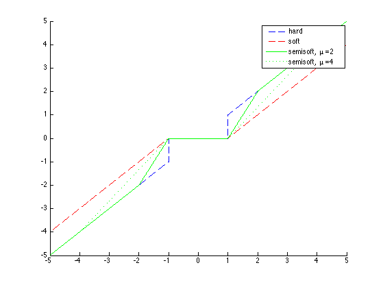
Semi-soft thresholding is a familly of non-linearities that interpolates between soft and hard thresholding. It uses both
a main threshold T and a secondary threshold T1=mu*T. When mu=1, the semi-soft thresholding performs a hard thresholding, whereas when mu=infty, it performs a soft thresholding.
T = 1;
v = linspace(-5,5,1024);
clf;
hold('on');
plot(v, perform_thresholding(v,T,'hard'), 'b--');
plot(v, perform_thresholding(v,T,'soft'), 'r--');
plot(v, perform_thresholding(v,[T 2*T],'semisoft'), 'g');
plot(v, perform_thresholding(v,[T 4*T],'semisoft'), 'g:');
legend('hard', 'soft', 'semisoft, \mu=2', 'semisoft, \mu=4');
hold('off');
Exercice 1: (check the solution) Compute the denoising SNR for different values of mu and different value of T. Important: to get good results, you should not threshold the low frequency residual.
exo1;
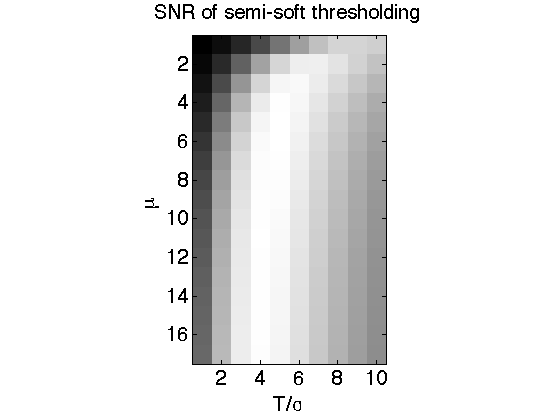
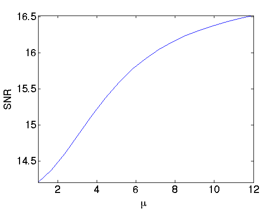
One can display, for each mu, the optimal SNR (obtained by testing many different T). For mu=1, one has the hard thresholding, which gives the worse SNR. The optimal SNR is atained here for mu approximately equal to 6.
err_mu = compute_min(err, 2);
clf;
plot(mulist, err_mu, '.-');
axis('tight');
set_label('\mu', 'SNR');
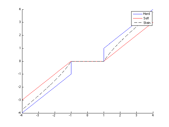
Soft and Stein Thresholding
Another way to achieve a tradeoff between hard and soft thresholding is to use a soft-squared thresholding non-linearity,
also named a Stein estimator.
We compute the thresholding curves.
T = 1;
v = linspace(-4,4,1024);
v_hard = v .* (abs(v)>T);
v_soft = v .* max( 1-T./abs(v), 0 );
v_stein = v .* max( 1-(T^2)./(v.^2), 0 );
We display the classical soft/hard thresholders.
clf;
hold('on');
plot(v, v_hard, 'b');
plot(v, v_soft, 'r');
plot(v, v_stein, 'k--');
hold('off');
legend('Hard', 'Soft', 'Stein');
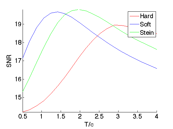
Exercice 2: (check the solution) Compare the performance of Soft and Stein thresholders, by determining the best threshold value.
exo2;