\[ \newcommand{\NN}{\mathbb{N}} \newcommand{\CC}{\mathbb{C}} \newcommand{\GG}{\mathbb{G}} \newcommand{\LL}{\mathbb{L}} \newcommand{\PP}{\mathbb{P}} \newcommand{\QQ}{\mathbb{Q}} \newcommand{\RR}{\mathbb{R}} \newcommand{\VV}{\mathbb{V}} \newcommand{\ZZ}{\mathbb{Z}} \newcommand{\FF}{\mathbb{F}} \newcommand{\KK}{\mathbb{K}} \newcommand{\UU}{\mathbb{U}} \newcommand{\EE}{\mathbb{E}} \newcommand{\Aa}{\mathcal{A}} \newcommand{\Bb}{\mathcal{B}} \newcommand{\Cc}{\mathcal{C}} \newcommand{\Dd}{\mathcal{D}} \newcommand{\Ee}{\mathcal{E}} \newcommand{\Ff}{\mathcal{F}} \newcommand{\Gg}{\mathcal{G}} \newcommand{\Hh}{\mathcal{H}} \newcommand{\Ii}{\mathcal{I}} \newcommand{\Jj}{\mathcal{J}} \newcommand{\Kk}{\mathcal{K}} \newcommand{\Ll}{\mathcal{L}} \newcommand{\Mm}{\mathcal{M}} \newcommand{\Nn}{\mathcal{N}} \newcommand{\Oo}{\mathcal{O}} \newcommand{\Pp}{\mathcal{P}} \newcommand{\Qq}{\mathcal{Q}} \newcommand{\Rr}{\mathcal{R}} \newcommand{\Ss}{\mathcal{S}} \newcommand{\Tt}{\mathcal{T}} \newcommand{\Uu}{\mathcal{U}} \newcommand{\Vv}{\mathcal{V}} \newcommand{\Ww}{\mathcal{W}} \newcommand{\Xx}{\mathcal{X}} \newcommand{\Yy}{\mathcal{Y}} \newcommand{\Zz}{\mathcal{Z}} \newcommand{\al}{\alpha} \newcommand{\la}{\lambda} \newcommand{\ga}{\gamma} \newcommand{\Ga}{\Gamma} \newcommand{\La}{\Lambda} \newcommand{\Si}{\Sigma} \newcommand{\si}{\sigma} \newcommand{\be}{\beta} \newcommand{\de}{\delta} \newcommand{\De}{\Delta} \renewcommand{\phi}{\varphi} \renewcommand{\th}{\theta} \newcommand{\om}{\omega} \newcommand{\Om}{\Omega} \renewcommand{\epsilon}{\varepsilon} \newcommand{\Calpha}{\mathrm{C}^\al} \newcommand{\Cbeta}{\mathrm{C}^\be} \newcommand{\Cal}{\text{C}^\al} \newcommand{\Cdeux}{\text{C}^{2}} \newcommand{\Cun}{\text{C}^{1}} \newcommand{\Calt}[1]{\text{C}^{#1}} \newcommand{\lun}{\ell^1} \newcommand{\ldeux}{\ell^2} \newcommand{\linf}{\ell^\infty} \newcommand{\ldeuxj}{{\ldeux_j}} \newcommand{\Lun}{\text{\upshape L}^1} \newcommand{\Ldeux}{\text{\upshape L}^2} \newcommand{\Lp}{\text{\upshape L}^p} \newcommand{\Lq}{\text{\upshape L}^q} \newcommand{\Linf}{\text{\upshape L}^\infty} \newcommand{\lzero}{\ell^0} \newcommand{\lp}{\ell^p} \renewcommand{\d}{\ins{d}} \newcommand{\Grad}{\text{Grad}} \newcommand{\grad}{\text{grad}} \renewcommand{\div}{\text{div}} \newcommand{\diag}{\text{diag}} \newcommand{\pd}[2]{ \frac{ \partial #1}{\partial #2} } \newcommand{\pdd}[2]{ \frac{ \partial^2 #1}{\partial #2^2} } \newcommand{\dotp}[2]{\langle #1,\,#2\rangle} \newcommand{\norm}[1]{|\!| #1 |\!|} \newcommand{\normi}[1]{\norm{#1}_{\infty}} \newcommand{\normu}[1]{\norm{#1}_{1}} \newcommand{\normz}[1]{\norm{#1}_{0}} \newcommand{\abs}[1]{\vert #1 \vert} \newcommand{\argmin}{\text{argmin}} \newcommand{\argmax}{\text{argmax}} \newcommand{\uargmin}[1]{\underset{#1}{\argmin}\;} \newcommand{\uargmax}[1]{\underset{#1}{\argmax}\;} \newcommand{\umin}[1]{\underset{#1}{\min}\;} \newcommand{\umax}[1]{\underset{#1}{\max}\;} \newcommand{\pa}[1]{\left( #1 \right)} \newcommand{\choice}[1]{ \left\{ \begin{array}{l} #1 \end{array} \right. } \newcommand{\enscond}[2]{ \left\{ #1 \;:\; #2 \right\} } \newcommand{\qandq}{ \quad \text{and} \quad } \newcommand{\qqandqq}{ \qquad \text{and} \qquad } \newcommand{\qifq}{ \quad \text{if} \quad } \newcommand{\qqifqq}{ \qquad \text{if} \qquad } \newcommand{\qwhereq}{ \quad \text{where} \quad } \newcommand{\qqwhereqq}{ \qquad \text{where} \qquad } \newcommand{\qwithq}{ \quad \text{with} \quad } \newcommand{\qqwithqq}{ \qquad \text{with} \qquad } \newcommand{\qforq}{ \quad \text{for} \quad } \newcommand{\qqforqq}{ \qquad \text{for} \qquad } \newcommand{\qqsinceqq}{ \qquad \text{since} \qquad } \newcommand{\qsinceq}{ \quad \text{since} \quad } \newcommand{\qarrq}{\quad\Longrightarrow\quad} \newcommand{\qqarrqq}{\quad\Longrightarrow\quad} \newcommand{\qiffq}{\quad\Longleftrightarrow\quad} \newcommand{\qqiffqq}{\qquad\Longleftrightarrow\qquad} \newcommand{\qsubjq}{ \quad \text{subject to} \quad } \newcommand{\qqsubjqq}{ \qquad \text{subject to} \qquad } \]

Dictionary Learning

Instead of using a fixed data representation such as wavelets or Fourier, one can learn the representation (the dictionary) to optimize the sparsity of the representation for a large class of exemplar.

Installing toolboxes and setting up the path.
Dictionary Learning as a Non-convex Optimization Problem
Patch Extraction
Update of the Coefficients \(X\)
Update the Dictionary \(D\)

Installing toolboxes and setting up the path.

You need to download the following files: signal toolbox and general toolbox.

You need to unzip these toolboxes in your working directory, so that you have toolbox_signal and toolbox_general in your directory.

For Scilab user: you must replace the Matlab comment '%' by its Scilab counterpart '//'.

Recommandation: You should create a text file named for instance numericaltour.sce (in Scilab) or numericaltour.m (in Matlab) to write all the Scilab/Matlab command you want to execute. Then, simply run exec('numericaltour.sce'); (in Scilab) or numericaltour; (in Matlab) to run the commands.

Execute this line only if you are using Matlab.

getd = @(p)path(p,path); % scilab users must *not* execute this

Then you can add the toolboxes to the path.

getd('toolbox_signal/');
getd('toolbox_general/');

Dictionary Learning as a Non-convex Optimization Problem

Given a set \(Y = (y_j)_{j=1}^m \in \RR^{n \times m} \) of \(m\) signals \(y_j \in \RR^m\), dictionary learning aims at finding the best dictionary \(D=(d_i)_{i=1}^p\) of \(p\) atoms \(d_i \in \RR^n\) to sparse code all the data.

In this numerical tour, we consider an application to image denoising, so that each \(y_j \in \RR^n\) is a patch of size \(n=w \times w\) extracted from the noisy image.

The idea of learning dictionaries to sparse code image patch was first proposed in:

Olshausen BA, and Field DJ., Emergence of Simple-Cell Receptive Field Properties by Learning a Sparse Code for Natural Images. Nature, 381: 607-609, 1996.

The sparse coding of a single data \(y=y_j\) for some \(j=1,\ldots,m\) is obtained by minimizing a \(\ell^0\) constrained optimization \[ \umin{ \norm{x}_0 \leq k } \frac{1}{2}\norm{y-Dx}^2 . \] where the \(\ell^0\) pseudo-norm of \(x \in \RR^p\) is \[ \norm{x}_0 = \abs{\enscond{i}{x(i) \neq 0}}. \]

The parameter \(k>0\) controls the amount of sparsity.

Dictionary learning performs an optimization both on the dictionary \(D\) and the set of coefficients \( X = (x_j)_{j=1}^m \in \RR^{p \times m} \) where, for \(j=1,\ldots,m\), \( x_j \) is the set of coefficients of the data \(y_j\). This joint optimization reads \[ \umin{ D \in \Dd, X \in \Xx_k } E(X,D) = \frac{1}{2}\norm{Y-DX}^2 = \frac{1}{2} \sum_{j=1}^m \norm{y_j - D x_j}^2. \]

The constraint set on \(D\) reads \[ \Dd = \enscond{D \in \RR^{n \times p} }{ \forall i=1,\ldots,p, \quad \norm{D_{\cdot,i}} \leq 1 }, \] (the columns of the dictionary are unit normalized). The sparsity constraint set on \(X\) reads \[ \Xx_k = \enscond{X \in \RR^{p \times m}}{ \forall j, \: \norm{X_{\cdot,j}}_0 \leq k }. \]

We propose to use a block-coordinate descent method to minimize \(E\): \[ X^{(\ell+1)} \in \uargmin{X \in \Xx_k} E(X,D^{(\ell)}), \] \[ D^{(\ell+1)} \in \uargmin{D \in \Dd} E(X^{(\ell+1)},D). \]

One can show the convergence of this minimization scheme, see for instance

P. Tseng, Convergence of Block Coordinate Descent Method for Nondifferentiable Minimization, J. Optim. Theory Appl., 109, 2001, 475-494.

We now define the parameter of the problem.

Width \(w\) of the patches.

if not(exist('w'))
    w = 10;
end

Dimension \(n= w \times w\) of the data to be sparse coded.

n = w*w;

Number of atoms \(p\) in the dictionary.

p = 2*n;

Number \(m\) of patches used for the training.

m = 20*p;

Target sparsity \(k\).

k = 4;

Patch Extraction

Since the learning is computationnaly intensive, one can only apply it to small patches extracted from an image.

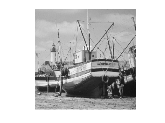
if not(exist('f'))
    f = rescale( crop(load_image('barb'),256) );
end
n0 = size(f,1);

Display the input image.

clf;
imageplot(clamp(f));

Random patch location.

q = 3*m;
x = floor( rand(1,1,q)*(n0-w) )+1;
y = floor( rand(1,1,q)*(n0-w) )+1;

Extract lots of patches \(y_j \in \RR^n\), and store them in a matrix \(Y=(y_j)_{j=1}^m\).

[dY,dX] = meshgrid(0:w-1,0:w-1);
Xp = repmat(dX,[1 1 q]) + repmat(x, [w w 1]);
Yp = repmat(dY,[1 1 q]) + repmat(y, [w w 1]);
Y = f(Xp+(Yp-1)*n0);
Y = reshape(Y, [n q]);

We remove the mean, since we are going to learn a dictionary of zero-mean and unit norm atom.

Y = Y - repmat( mean(Y), [n 1] );

Only keep those with largest energy.

[tmp,I] = sort(sum(Y.^2), 'descend');
Y = Y(:,I(1:m));

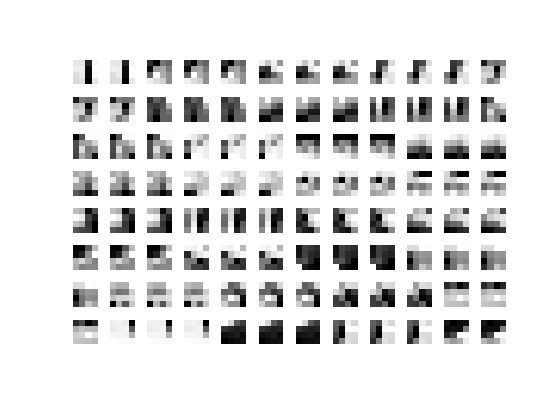
We consider a dictionary \(D \in \RR^{n \times p} \) of \(p \geq n\) atoms in \(\RR^n\). The initial dictionary \(D\) is computed by a random selection of patches, and we normalize them to be unit-norm.

ProjC = @(D)D ./ repmat( sqrt(sum(D.^2)), [w^2, 1] );
sel = randperm(m); sel = sel(1:p);
D0 = ProjC( Y(:,sel) );
D = D0;

Display the initial dictionary.

clf;
plot_dictionnary(D, [], [8 12]);

Update of the Coefficients \(X\)

The optimization on the coefficients \(X\) requires, for each \(y_j = Y_{\cdot,j}\) to compute \(x_j = X_{\cdot,j}\) that solves \[ \umin{ \norm{x_j}_0 \leq k } \frac{1}{2} \norm{y-D x_j}^2. \]

This is a non-smooth and non-convex minimization, that can be shown to be NP-hard. A heuristic to solve this method is to compute a stationary point of the energy using the Foward-Backward iterative scheme (projected gradient descent): \[ x_j \leftarrow \text{Proj}_{\Xx_k}\pa{ x_j - \tau D^* ( D x_j - y ) } \qwhereq \tau < \frac{2}{\norm{D D^*}}. \]

Denoting \(\abs{\bar x(1)} \leq \ldots \leq \abs{\bar x(n)}\) the ordered magnitudes of a vector \( x \in \RR^n \), the orthogonal projector on \(\Xx_k\) reads \(z = \text{Proj}_{\Xx_k}(x)\) with \[ \forall i=1,\ldots,n, \quad z(i) = \choice{ x(i) \qifq \abs{x(i)} \geq \abs{\bar x(k)}, \\ z(i) = 0 \quad \text{otherwise}. } \]

select = @(A,k)repmat(A(k,:), [size(A,1) 1]);
ProjX = @(X,k)X .* (abs(X) >= select(sort(abs(X), 'descend'),k));

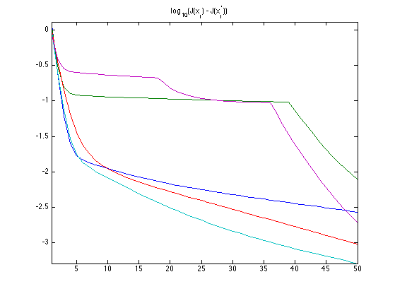
Exercice 1: (check the solution) Perform the iterative hard thresholding, and display the decay of the energy \(J(x_j) = \norm{y_j-D x_j}^2\) for several \(j\). Remark: note that the iteration can be performed in parallel on all \(x_j\).

exo1;

Update the Dictionary \(D\)

Once the sparse coefficients \(X\) have been computed, one can udpate the dictionary. This is achieve by performing the minimization \[ \umin{D \in \Dd} \frac{1}{2}\norm{Y-D X}^2. \]

One can perform this minimization with a projected gradient descent \[ D \leftarrow \text{Proj}_{\Cc}\pa{ D - \tau (DX - Y)X^* } \] where \( \tau < 2/\norm{XX^*}. \)

Note that the orthogonal projector \(\text{Proj}_{\Cc}\) is implemented in the function ProjC already defined.

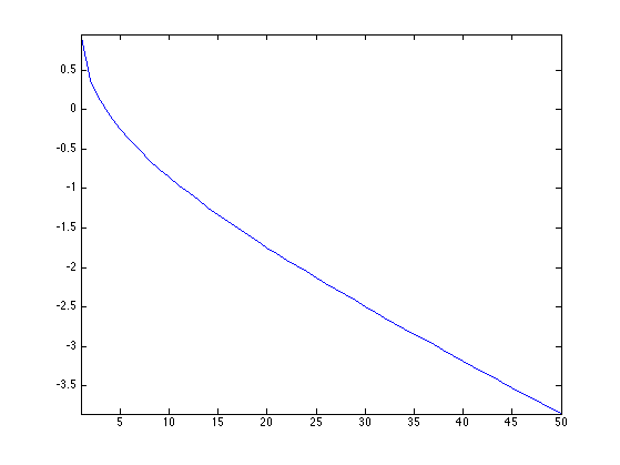
Exercice 2: (check the solution) Perform this gradient descent, and monitor the decay of the energy.

exo2;

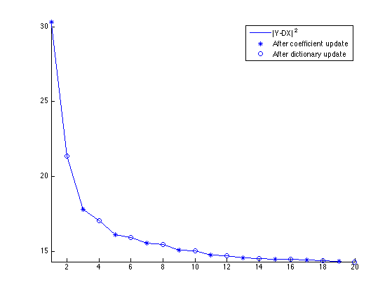
Exercice 3: (check the solution) Perform the dictionary learning by iterating between sparse coding and dictionary update.

exo3;

Display the dictionary.

clf;
plot_dictionnary(D,X, [8 12]);

Index exceeds matrix dimensions.

Error in plot_dictionnary (line 69)
vmax = max( max( abs( D(:,I(1:prod(nb))) ) ) );

Error in index (line 256)
plot_dictionnary(D,X, [8 12]);