\[ \newcommand{\NN}{\mathbb{N}} \newcommand{\CC}{\mathbb{C}} \newcommand{\GG}{\mathbb{G}} \newcommand{\LL}{\mathbb{L}} \newcommand{\PP}{\mathbb{P}} \newcommand{\QQ}{\mathbb{Q}} \newcommand{\RR}{\mathbb{R}} \newcommand{\VV}{\mathbb{V}} \newcommand{\ZZ}{\mathbb{Z}} \newcommand{\FF}{\mathbb{F}} \newcommand{\KK}{\mathbb{K}} \newcommand{\UU}{\mathbb{U}} \newcommand{\EE}{\mathbb{E}} \newcommand{\Aa}{\mathcal{A}} \newcommand{\Bb}{\mathcal{B}} \newcommand{\Cc}{\mathcal{C}} \newcommand{\Dd}{\mathcal{D}} \newcommand{\Ee}{\mathcal{E}} \newcommand{\Ff}{\mathcal{F}} \newcommand{\Gg}{\mathcal{G}} \newcommand{\Hh}{\mathcal{H}} \newcommand{\Ii}{\mathcal{I}} \newcommand{\Jj}{\mathcal{J}} \newcommand{\Kk}{\mathcal{K}} \newcommand{\Ll}{\mathcal{L}} \newcommand{\Mm}{\mathcal{M}} \newcommand{\Nn}{\mathcal{N}} \newcommand{\Oo}{\mathcal{O}} \newcommand{\Pp}{\mathcal{P}} \newcommand{\Qq}{\mathcal{Q}} \newcommand{\Rr}{\mathcal{R}} \newcommand{\Ss}{\mathcal{S}} \newcommand{\Tt}{\mathcal{T}} \newcommand{\Uu}{\mathcal{U}} \newcommand{\Vv}{\mathcal{V}} \newcommand{\Ww}{\mathcal{W}} \newcommand{\Xx}{\mathcal{X}} \newcommand{\Yy}{\mathcal{Y}} \newcommand{\Zz}{\mathcal{Z}} \newcommand{\al}{\alpha} \newcommand{\la}{\lambda} \newcommand{\ga}{\gamma} \newcommand{\Ga}{\Gamma} \newcommand{\La}{\Lambda} \newcommand{\Si}{\Sigma} \newcommand{\si}{\sigma} \newcommand{\be}{\beta} \newcommand{\de}{\delta} \newcommand{\De}{\Delta} \renewcommand{\phi}{\varphi} \renewcommand{\th}{\theta} \newcommand{\om}{\omega} \newcommand{\Om}{\Omega} \renewcommand{\epsilon}{\varepsilon} \newcommand{\Calpha}{\mathrm{C}^\al} \newcommand{\Cbeta}{\mathrm{C}^\be} \newcommand{\Cal}{\text{C}^\al} \newcommand{\Cdeux}{\text{C}^{2}} \newcommand{\Cun}{\text{C}^{1}} \newcommand{\Calt}[1]{\text{C}^{#1}} \newcommand{\lun}{\ell^1} \newcommand{\ldeux}{\ell^2} \newcommand{\linf}{\ell^\infty} \newcommand{\ldeuxj}{{\ldeux_j}} \newcommand{\Lun}{\text{\upshape L}^1} \newcommand{\Ldeux}{\text{\upshape L}^2} \newcommand{\Lp}{\text{\upshape L}^p} \newcommand{\Lq}{\text{\upshape L}^q} \newcommand{\Linf}{\text{\upshape L}^\infty} \newcommand{\lzero}{\ell^0} \newcommand{\lp}{\ell^p} \renewcommand{\d}{\ins{d}} \newcommand{\Grad}{\text{Grad}} \newcommand{\grad}{\text{grad}} \renewcommand{\div}{\text{div}} \newcommand{\diag}{\text{diag}} \newcommand{\pd}[2]{ \frac{ \partial #1}{\partial #2} } \newcommand{\pdd}[2]{ \frac{ \partial^2 #1}{\partial #2^2} } \newcommand{\dotp}[2]{\langle #1,\,#2\rangle} \newcommand{\norm}[1]{|\!| #1 |\!|} \newcommand{\normi}[1]{\norm{#1}_{\infty}} \newcommand{\normu}[1]{\norm{#1}_{1}} \newcommand{\normz}[1]{\norm{#1}_{0}} \newcommand{\abs}[1]{\vert #1 \vert} \newcommand{\argmin}{\text{argmin}} \newcommand{\argmax}{\text{argmax}} \newcommand{\uargmin}[1]{\underset{#1}{\argmin}\;} \newcommand{\uargmax}[1]{\underset{#1}{\argmax}\;} \newcommand{\umin}[1]{\underset{#1}{\min}\;} \newcommand{\umax}[1]{\underset{#1}{\max}\;} \newcommand{\pa}[1]{\left( #1 \right)} \newcommand{\choice}[1]{ \left\{ \begin{array}{l} #1 \end{array} \right. } \newcommand{\enscond}[2]{ \left\{ #1 \;:\; #2 \right\} } \newcommand{\qandq}{ \quad \text{and} \quad } \newcommand{\qqandqq}{ \qquad \text{and} \qquad } \newcommand{\qifq}{ \quad \text{if} \quad } \newcommand{\qqifqq}{ \qquad \text{if} \qquad } \newcommand{\qwhereq}{ \quad \text{where} \quad } \newcommand{\qqwhereqq}{ \qquad \text{where} \qquad } \newcommand{\qwithq}{ \quad \text{with} \quad } \newcommand{\qqwithqq}{ \qquad \text{with} \qquad } \newcommand{\qforq}{ \quad \text{for} \quad } \newcommand{\qqforqq}{ \qquad \text{for} \qquad } \newcommand{\qqsinceqq}{ \qquad \text{since} \qquad } \newcommand{\qsinceq}{ \quad \text{since} \quad } \newcommand{\qarrq}{\quad\Longrightarrow\quad} \newcommand{\qqarrqq}{\quad\Longrightarrow\quad} \newcommand{\qiffq}{\quad\Longleftrightarrow\quad} \newcommand{\qqiffqq}{\qquad\Longleftrightarrow\qquad} \newcommand{\qsubjq}{ \quad \text{subject to} \quad } \newcommand{\qqsubjqq}{ \qquad \text{subject to} \qquad } \]

Gradient Descent Methods

This tour explores the use of gradient descent method for unconstrained and constrained optimization of a smooth function

Installing toolboxes and setting up the path.
Gradient Descent for Unconstrained Problems
Gradient Descent in 2-D
Gradient and Divergence of Images
Gradient Descent in Image Processing
Constrained Optimization Using Projected Gradient Descent

Installing toolboxes and setting up the path.

You need to download the following files: signal toolbox and general toolbox.

You need to unzip these toolboxes in your working directory, so that you have toolbox_signal and toolbox_general in your directory.

For Scilab user: you must replace the Matlab comment '%' by its Scilab counterpart '//'.

Recommandation: You should create a text file named for instance numericaltour.sce (in Scilab) or numericaltour.m (in Matlab) to write all the Scilab/Matlab command you want to execute. Then, simply run exec('numericaltour.sce'); (in Scilab) or numericaltour; (in Matlab) to run the commands.

Execute this line only if you are using Matlab.

getd = @(p)path(p,path); % scilab users must *not* execute this

Then you can add the toolboxes to the path.

getd('toolbox_signal/');
getd('toolbox_general/');

Gradient Descent for Unconstrained Problems

We consider the problem of finding a minimum of a function \(f\), hence solving \[ \umin{x \in \RR^d} f(x) \] where \(f : \RR^d \rightarrow \RR\) is a smooth function.

Note that the minimum is not necessarily unique. In the general case, \(f\) might exhibit local minima, in which case the proposed algorithms is not expected to find a global minimizer of the problem. In this tour, we restrict our attention to convex function, so that the methods will converge to a global minimizer.

The simplest method is the gradient descent, that computes \[ x^{(k+1)} = x^{(k)} - \tau_k \nabla f(x^{(k)}), \] where \(\tau_k>0\) is a step size, and \(\nabla f(x) \in \RR^d\) is the gradient of \(f\) at the point \(x\), and \(x^{(0)} \in \RR^d\) is any initial point.

In the convex case, if \(f\) is of class \(C^2\), in order to ensure convergence, the step size should satisfy \[ 0 < \tau_k < \frac{2}{ \sup_x \norm{Hf(x)} } \] where \(Hf(x) \in \RR^{d \times d}\) is the Hessian of \(f\) at \(x\) and \( \norm{\cdot} \) is the spectral operator norm (largest eigenvalue).

Gradient Descent in 2-D

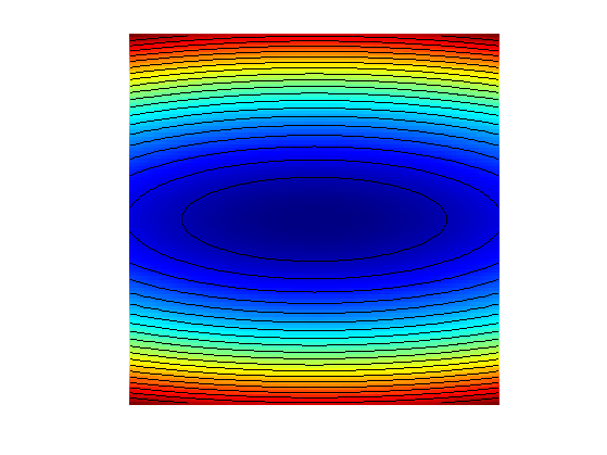
We consider a simple problem, corresponding to the minimization of a 2-D quadratic form \[ f(x) = \frac{1}{2} \pa{ x_1^2 + \eta x_2^2, } \] where \( \eta>0 \) controls the anisotropy, and hence the difficulty, of the problem.

Anisotropy parameter \(\eta\).

eta = 10;

Function \(f\).

f = @(x)( x(1)^2 + eta*x(2)^2 ) /2;

Background image of the function.

t = linspace(-.7,.7,101);
[u,v] = meshgrid(t,t);
F = ( u.^2 + eta*v.^2 )/2 ;

Display the function as a 2-D image.

clf; hold on;
imagesc(t,t,F); colormap jet(256);
contour(t,t,F, 20, 'k');
axis off; axis equal;

Gradient.

Gradf = @(x)[x(1); eta*x(2)];

The step size should satisfy \(\tau_k < 2/\eta\). We use here a constrant step size.

tau = 1.8/eta;

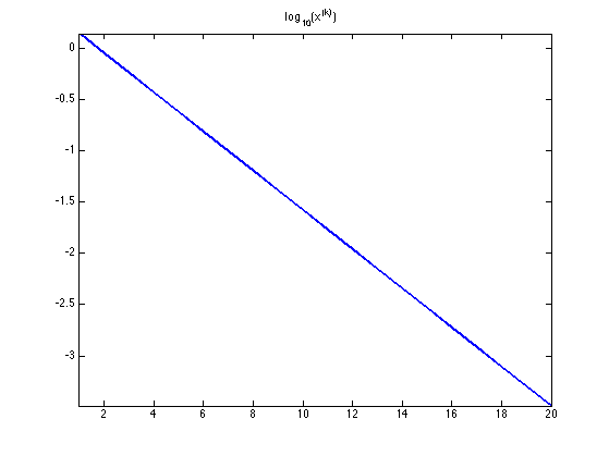
Exercice 1: (check the solution) Perform the gradient descent using a fixed step size \(\tau_k=\tau\). Display the decay of the energy \(f(x^{(k)})\) through the iteration. Save the iterates so that X(:,k) corresponds to \(x^{(k)}\).

exo1;

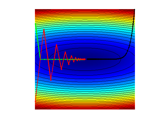
Display the iterations.

clf; hold on;
imagesc(t,t,F); colormap jet(256);
contour(t,t,F, 20, 'k');
h = plot(X(1,:), X(2,:), 'k.-');
set(h, 'LineWidth', 2);
set(h, 'MarkerSize', 15);
axis off; axis equal;

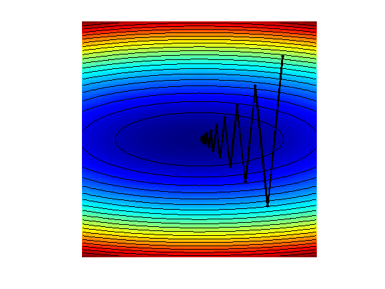
Exercice 2: (check the solution) Display the iteration for several different step sizes.

exo2;

Gradient and Divergence of Images

Local differential operators like gradient, divergence and laplacian are the building blocks for variational image processing.

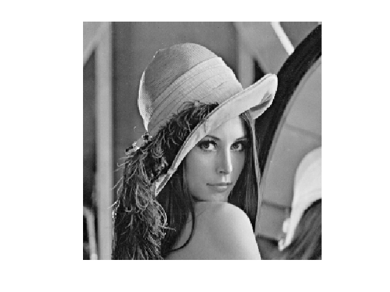
Load an image \(x_0 \in \RR^N\) of \(N=n \times n\) pixels.

n = 256;
x0 = rescale( load_image('lena',n) );

Display it.

clf;
imageplot(x0);

For a continuous function \(g\), the gradient reads \[ \nabla g(s) = \pa{ \pd{g(s)}{s_1}, \pd{g(s)}{s_2} } \in \RR^2. \] (note that here, the variable \(s\) denotes the 2-D spacial position).

We discretize this differential operator on a discrete image \(x \in \RR^N\) using first order finite differences. \[ (\nabla x)_i = ( x_{i_1,i_2}-x_{i_1-1,i_2}, x_{i_1,i_2}-x_{i_1,i_2-1} ) \in \RR^2. \] Note that for simplity we use periodic boundary conditions.

Compute its gradient, using finite differences.

grad = @(x)cat(3, x-x([end 1:end-1],:), x-x(:,[end 1:end-1]));

One thus has \( \nabla : \RR^N \mapsto \RR^{N \times 2}. \)

v = grad(x0);

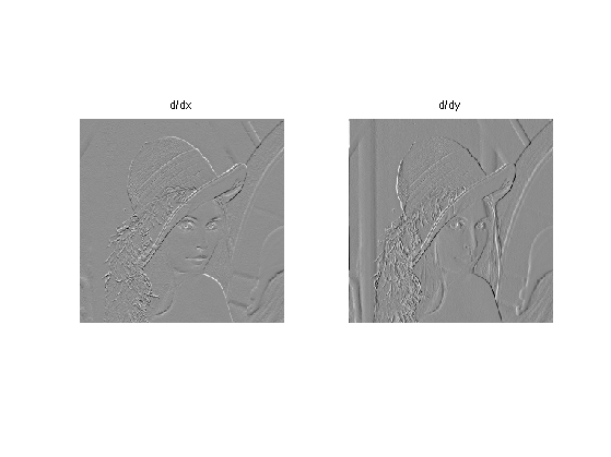
One can display each of its components.

clf;
imageplot(v(:,:,1), 'd/dx', 1,2,1);
imageplot(v(:,:,2), 'd/dy', 1,2,2);

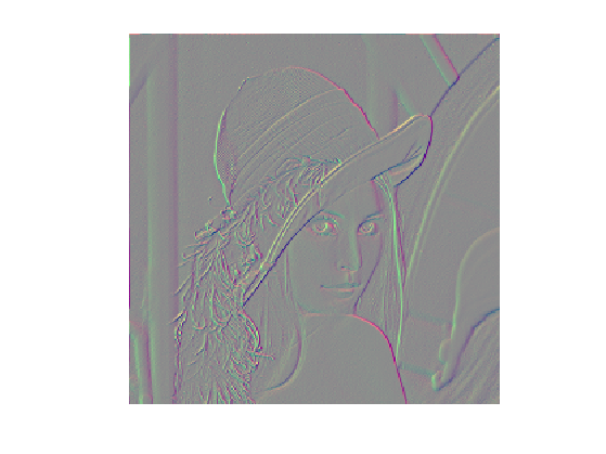
One can also display it using a color image.

clf;
imageplot(v);

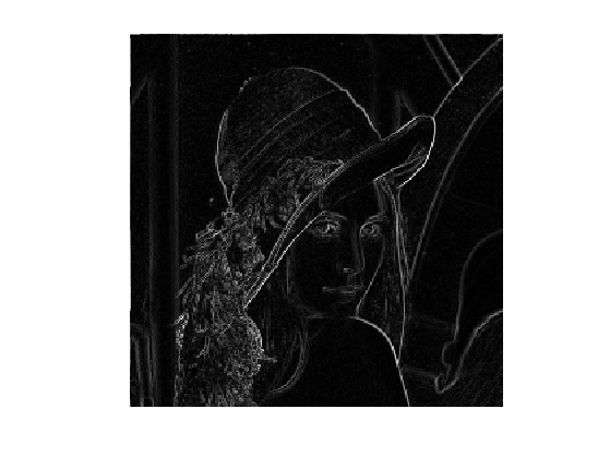
One can display its magnitude \(\norm{(\nabla x)_i}\), which is large near edges.

clf;
imageplot( sqrt( sum3(v.^2,3) ) );

The divergence operator maps vector field to images. For continuous vector fields \(v(s) \in \RR^2\), it is defined as \[ \text{div}(v)(s) = \pd{v_1(s)}{s_1} + \pd{v_2(s)}{s_2} \in \RR. \] (note that here, the variable \(s\) denotes the 2-D spacial position). It is minus the adjoint of the gadient, i.e. \(\text{div} = - \nabla^*\).

It is discretized, for \(v=(v^1,v^2)\) as \[ \text{div}(v)_i = v^1_{i_1+1,i_2} - v^1_{i_1,i_2} + v^2_{i_1,i_2+1} - v^2_{i_1,i_2} . \]

div = @(v)v([2:end 1],:,1)-v(:,:,1) + v(:,[2:end 1],2)-v(:,:,2);

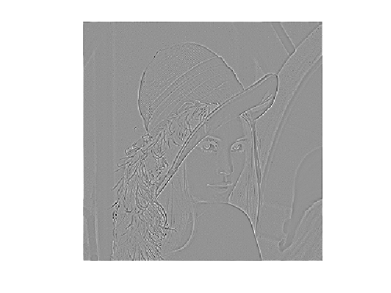
The Laplacian operatore is defined as \(\Delta=\text{div} \circ \nabla = -\nabla^* \circ \nabla\). It is thus a negative symmetric operator.

delta = @(x)div(grad(x));

Display \(\Delta x_0\).

clf;
imageplot(delta(x0));

Check that the relation \( \norm{\nabla x} = - \dotp{\Delta x}{x}. \)

dotp = @(a,b)sum(a(:).*b(:));
fprintf('Should be 0: %.3i\n', dotp(grad(x0), grad(x0)) + dotp(delta(x0),x0) );

Should be 0: 000

Gradient Descent in Image Processing

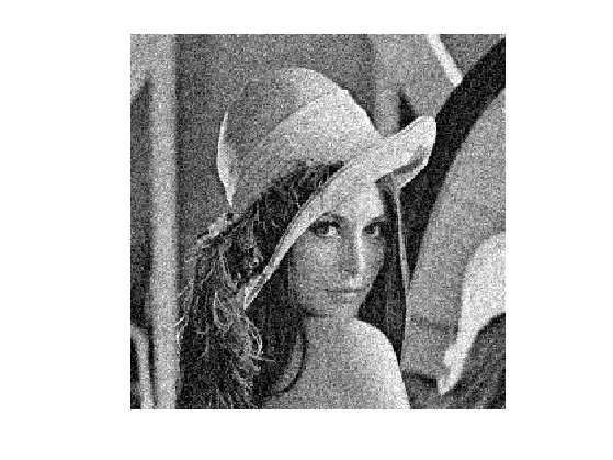
We consider now the problem of denoising an image \(y \in \RR^d\) where \(d = n \times n\) is the number of pixels (\(n\) being the number of rows/columns in the image).

Add noise to the original image, to simulate a noisy image.

sigma = .1;
y = x0 + randn(n)*sigma;

Display the noisy image \(y\).

clf;
imageplot(clamp(y));

Denoising is obtained by minimizing the following functional \[ \umin{x \in \RR^d} f(x) = \frac{1}{2} \norm{y-x}^2 + \la J_\epsilon(x) \] where \(J_\epsilon(x)\) is a smoothed total variation of the image. \[ J_\epsilon(x) = \sum_i \norm{ (G x)_i }_{\epsilon} \] where \( (Gx)_i \in \RR^2 \) is an approximation of the gradient of \(x\) at pixel \(i\) and for \(u \in \RR^2\), we use the following smoothing of the \(L^2\) norm in \(\RR^2\) \[ \norm{u}_\epsilon = \sqrt{ \epsilon^2 + \norm{u}^2 }, \] for a small value of \(\epsilon>0\).

The gradient of the functional read \[ \nabla f(x) = x-y + \lambda \nabla J_\epsilon(x) \] where the gradient of the smoothed TV norm is \[ \nabla J_\epsilon(x)_i = G^*( u ) \qwhereq u_i = \frac{ (G x)_i }{\norm{ (G x)_i }_\epsilon} \] where \(G^*\) is the adjoint operator of \(G\) which corresponds to minus a discretized divergence.

Value for \(\lambda\).

lambda = .3/5;

Value for \(\epsilon\).

epsilon = 1e-3;

TV norm.

NormEps = @(u,epsilon)sqrt(epsilon^2 + sum(u.^2,3));
J = @(x,epsilon)sum(sum(NormEps(grad(x),epsilon)));

Function \(f\) to minimize.

f = @(y,x,epsilon)1/2*norm(x-y,'fro')^2 + lambda*J(x,epsilon);

Gradient of \(J_\epsilon\). Note that div implement \(-G^*\).

Normalize = @(u,epsilon)u./repmat(NormEps(u,epsilon), [1 1 2]);
GradJ = @(x,epsilon)-div( Normalize(grad(x),epsilon) );

Gradient of the functional.

Gradf = @(y,x,epsilon)x-y+lambda*GradJ(x,epsilon);

The step size should satisfy \[ 0 < \tau_k < \frac{2}{ 1 + 4 \lambda / \epsilon }. \] Here we use a slightly larger step size, which still work in practice.

tau = 1.8/( 1 + lambda*8/epsilon );
tau = tau*4;

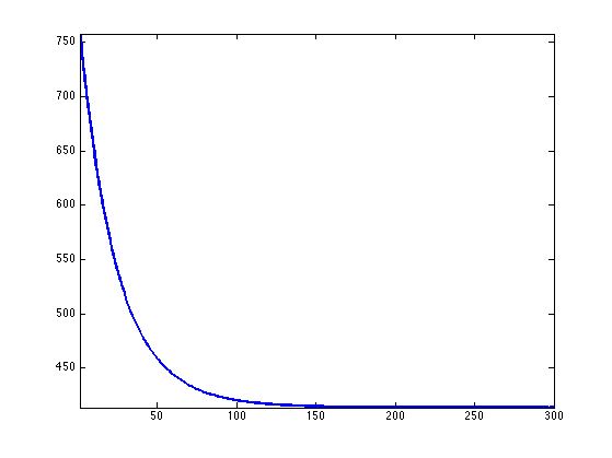
Exercice 3: (check the solution) Implement the gradient descent. Monitor the decay of \(f\) through the iterations.

exo3;

Display the resulting denoised image.

clf;
imageplot(clamp(x));

Constrained Optimization Using Projected Gradient Descent

We consider a linear imaging operator \(\Phi : x \mapsto \Phi(x)\) that maps high resolution images to low dimensional observations. Here we consider a pixel masking operator, that is diagonal over the spacial domain.

To emphasis the effect of the TV functional, we use a simple geometric image.

n = 64;
name = 'square';
x0 = load_image(name,n);

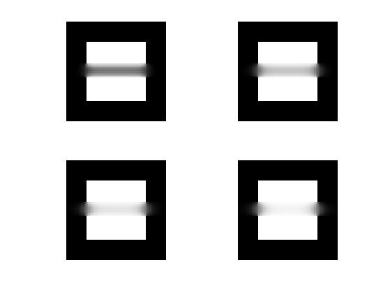
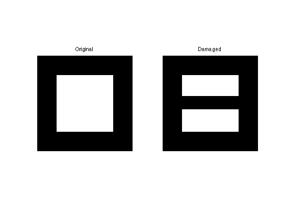
We consider here the inpainting problem. This simply corresponds to a masking operator. Here we remove the central part of the image.

a = 4;
Lambda = ones(n);
Lambda(end/2-a:end/2+a,:) = 0;

Masking operator \( \Phi \). Note that it is symmetric, i.e. \(\Phi^*=\Phi\)

Phi  = @(x)x.*Lambda;
PhiS = @(x)Phi(x);

Noiseless observations \(y=\Phi x_0\).

y = Phi(x0);

Display.

clf;
imageplot(x0, 'Original', 1,2,1);
imageplot(y, 'Damaged', 1,2,2);

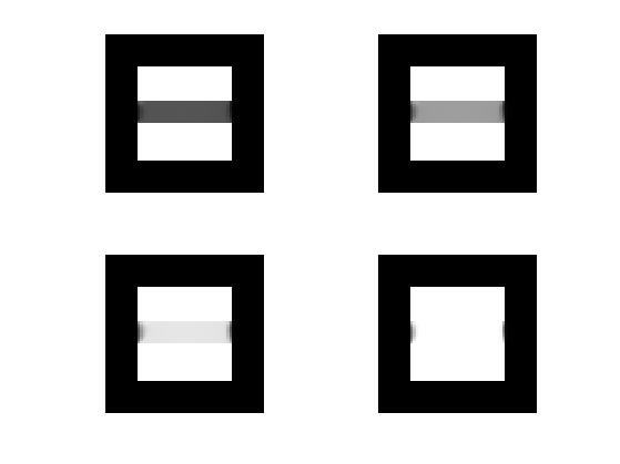
We want to solve the noiseless inverse problem \(y=\Phi f\) using a total variation regularization: \[ \umin{ y=\Phi x } J_\epsilon(x). \] We use the following projected gradient descent \[ x^{(k+1)} = \text{Proj}_{\Hh}( x^{(k)} - \tau_k \nabla J_{\epsilon}(x^{(k)}) ) \] where \(\text{Proj}_{\Hh}\) is the orthogonal projection on the set of linear constraint \(\Phi x = y\), and is easy to compute for inpainting

ProjH = @(x,y) x + PhiS( y - Phi(x) );

Exercice 4: (check the solution) Display the evolution of the inpainting process.

exo4;

Exercice 5: (check the solution) Try with several values of \(\epsilon\).

exo5;